Philadelphia Housing Price Prediction

Improving Property Tax Assessments

BBQ Chips Inc.

Research Question

• What factors (structural, census, spatial etc. ) most significantly impact the predictive accuracy of house price models?

Sub-questions:

• “Which factors are most influential in determining house price prediction outcomes?”

• “To what extent are house prices predictable, and to what extent are they driven by unobservable factors?”

• “Does the predictive performance of the model remain consistent across neighborhoods of varying wealth levels?”

Data Sources

• Census ACS (American Community Survey, 2022)

• OpenDataPhilly

  • Philadelphia Properties and Current Assessments (2023-2024)

  • Crime Incidents: Citywide crime incident reports

  • Universities: Spatial locations of educational institutions

  • Neighborhood Boundaries: Official neighborhood and planning district shapefiles

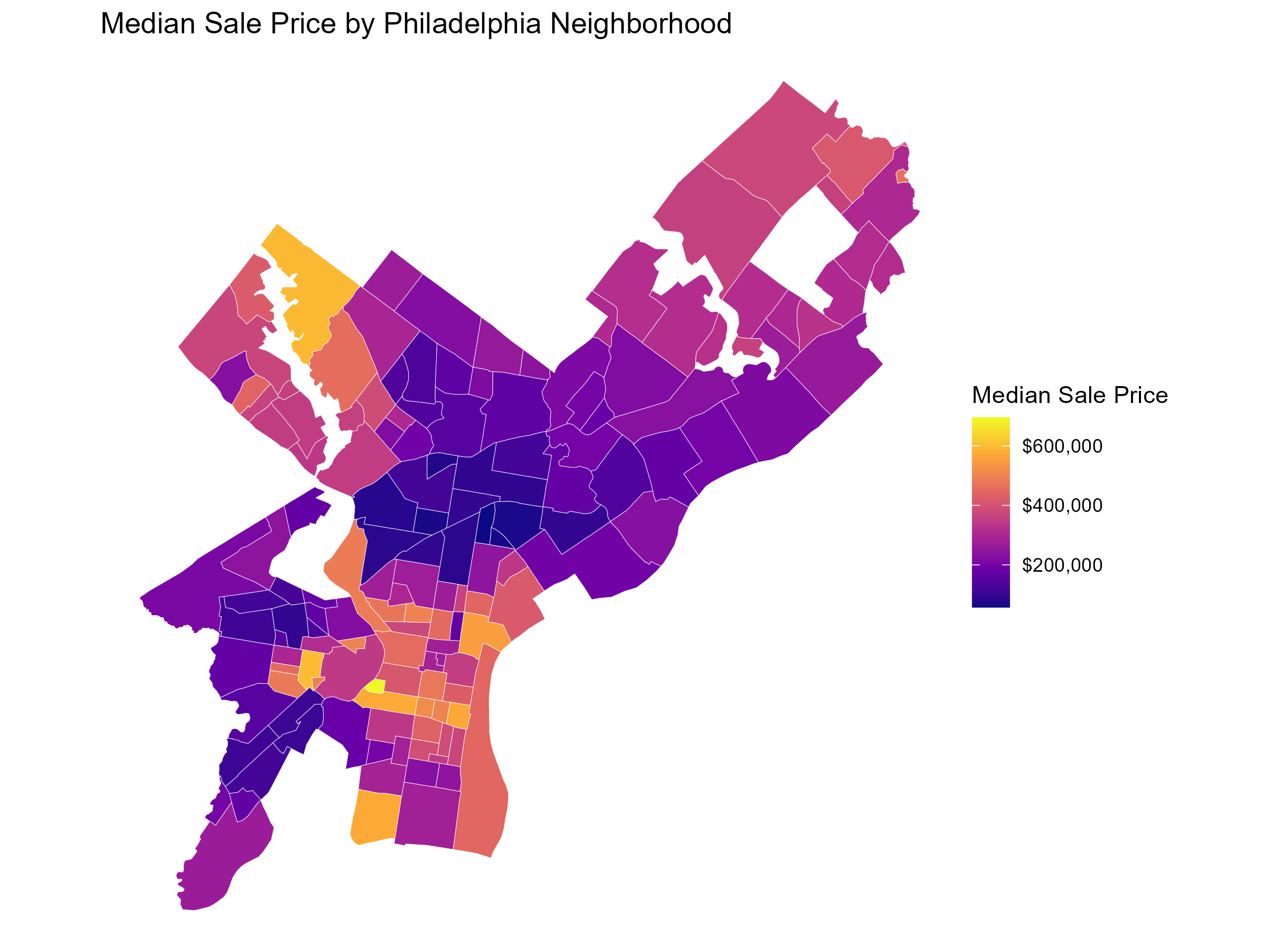
Exploratory Data Analysis

Model Building

Build models progressively:

Model 1: Structural features only
- number of bathrooms, livable area (logged), garage spaces, house age (Quadratic Effect), exterior condition

Model 2: Census variables
- median_income, percentage of bachelor, percentage of poverty

Model 3: Spatial features
- nearest college, number of nearby crime

Model 4: Interactions and fixed effects
- neighborhood wealthy (interact with livable area)

Comparison table

Model Performance Improves with Each Layer

Model	CV RMSE (log)	R²
Structural Only	0.61	0.35
+ Census	0.50	0.57
+ Spatial	0.49	0.58
+ Interactions/FE	0.48	0.59

Fourth Model RMSE: $154,200

Model Validation

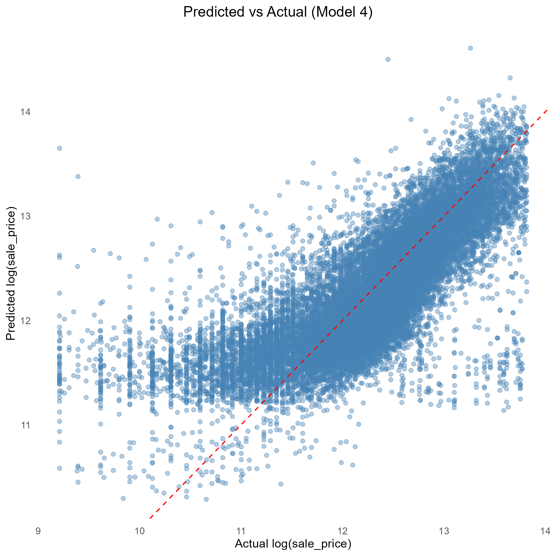
Model 4 Performance Summary

• Adjusted R² = 0.591 → explains nearly 59% of variation in sale price
• Major improvement from Model 1 (R² = 0.35) after adding neighborhood and spatial features

Key Takeaway

The final interaction model effectively captures both structural and contextual determinants of housing prices in Philadelphia, combining property-level features with socioeconomic and spatial characteristics.

Which Features Matter Most?

Feature	Direction	Interpretation
Living area	↑	Strongest driver of housing price
Age + Age²	↓ then ↑	U-shaped pattern — older historic homes regain value
Exterior good	↑	Maintenance condition positively impacts price
Median income / Education	↑	Socioeconomic context drives demand
Poverty rate / Crime	↓	Negative neighborhood effects
Interaction: Living area × Wealthy neighborhood	↓	Larger homes add less

Equity Concerns

• Price determinants vary by neighborhood wealth
  
• Model performs best in mid-range markets, less stable in low-value areas
  
• Hardest Neighborhoods to predict: Nicetown, Fairhill, and Upper Kensington
  
• Introduce spatial autoregressive or equity-weighted models

Model Limitations and Next Steps

Key Limitations

• Spatial autocorrelation: Some clustering remains in residuals — spatial lag or error models could improve performance.
  
• Omitted variables: Missing data on school quality, zoning, renovation, and accessibility likely affect price variation.
  
• Equity bias: Predictive accuracy varies by neighborhood wealth; uniform valuation may reinforce systemic disparities.

Next Steps

• Consider other spatial features to help magnify spatial patterns
• Extend analysis with temporal dimension (panel data) to capture price dynamics over time.

Policy Recommendations

• Risk of encoding structural inequalities from historical disinvestment

• Introduce equity-weighted adjustments or localized calibration for underrepresented areas

• Use residual maps to guide targeted reinvestment and housing policy

Conclusion

• Limitations:
  • observations omitted during dating cleaning
  • equity bias

Thank you for listening

Any questions?