Introduction to Linear Regression

Week 5: MUSA 5080

Dr. Elizabeth Delmelle

2025-10-06

Opening Question

Scenario: You’re advising a state agency on resource allocation.

Some counties have sparse data. Can you predict their median income using data from counties with better measurements?

Broader question: How do we make informed predictions when we don’t have complete information?

Today’s Roadmap

The Statistical Learning Framework: What are we actually doing?
Two goals: Understanding relationships vs Making predictions
Building your first model with PA census data
Model evaluation: How do we know if it’s any good?
Checking assumptions: When can we trust the model?
Improving predictions: Transformations, multiple variables

Part 1: The Statistical Learning Framework

The General Problem

We observe data: counties, income, population, education, etc.

We believe there’s some relationship between these variables.

Statistical learning = a set of approaches for estimating that relationship

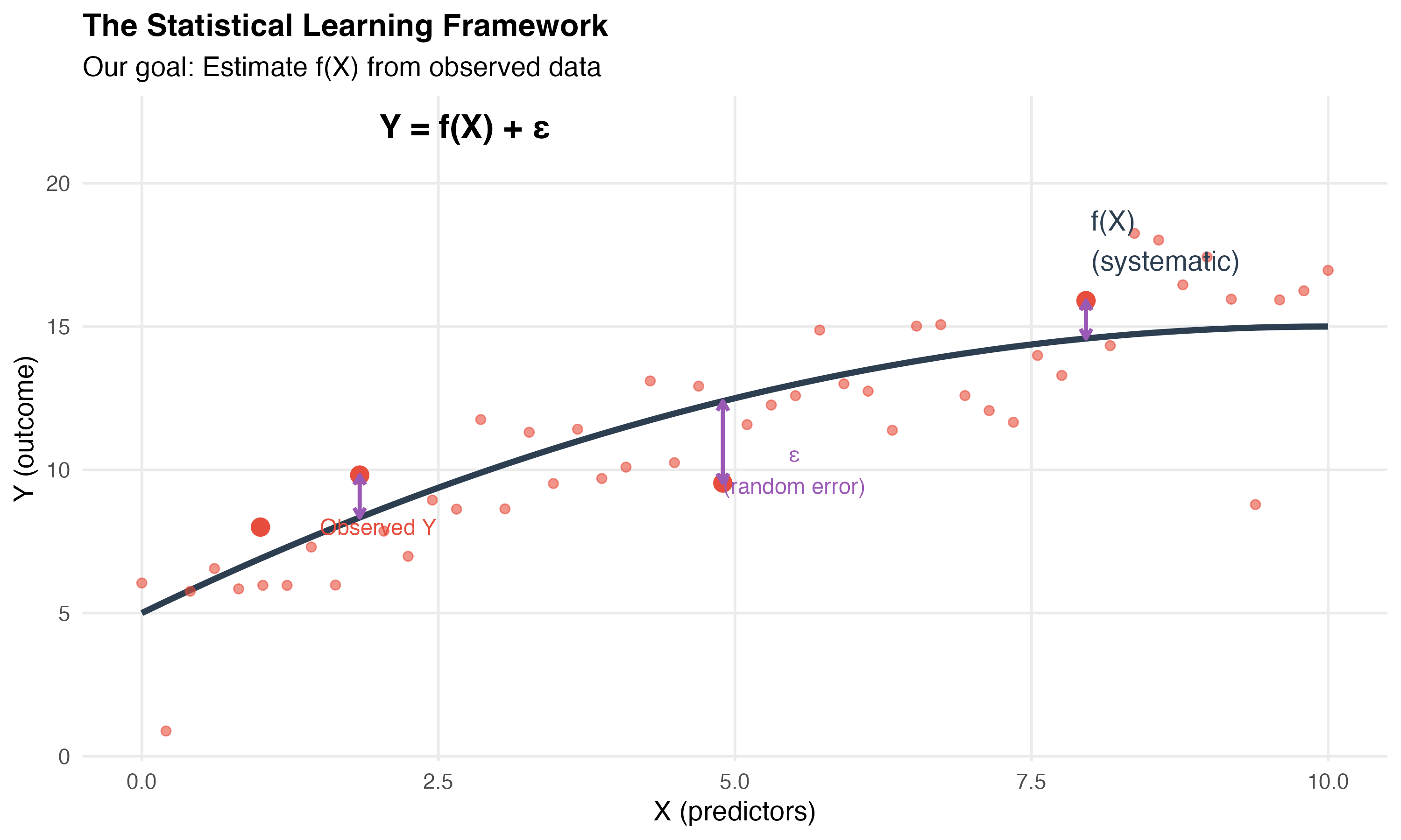
Formalizing the Relationship

For any quantitative response Y and predictors X₁, X₂, … Xₚ:

\[Y = f(X) + \epsilon\]

Where:

f = the systematic information X provides about Y
ε = random error (irreducible)

What is f?

f represents the true relationship between predictors and outcome

It’s fixed but unknown
It’s what we’re trying to estimate
Different X values produce different Y values through f

Example:

Y = median income
X = population, education, poverty rate
f = the way these factors systematically relate to income

Why Estimate f?

Two main reasons:

1. Prediction

Estimate Y for new observations
Don’t necessarily care about the exact form of f
Focus: accuracy of predictions

2. Inference

Understand how X affects Y
Which predictors matter?
What’s the nature of the relationship?
Focus: interpreting the model

How Do We Estimate f?

Two broad approaches:

Parametric Methods

Make an assumption about the functional form (e.g., linear)
Reduces problem to estimating a few parameters
Easier to interpret
This is what we’ll focus on

Non-Parametric Methods

Don’t assume a specific form
More flexible
Require more data
Harder to interpret

Parametric vs. Non-Parametric

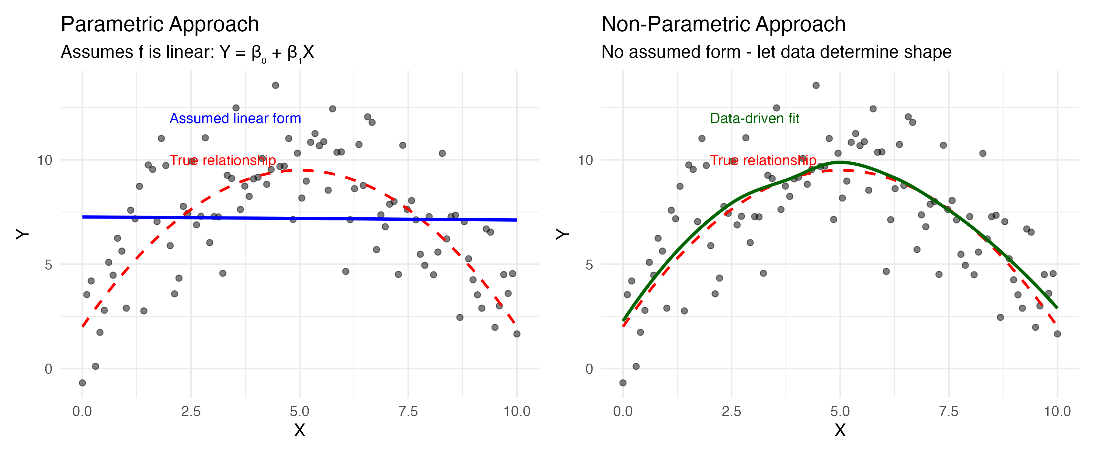
Key difference:

Parametric (blue): We assume f is linear, then estimate β₀ and β₁
Non-parametric (green): We let the data determine the shape of f

What about deep learning?

Neural networks are technically parametric (millions of parameters!), but achieve flexibility through parameter quantity rather than assuming a rigid form. We won’t cover them in this course, but they follow the same Y = f(X) + ε framework.

Parametric Approach: Linear Regression

The assumption: Relationship between X and Y is linear

\[Y \approx \beta_0 + \beta_1X_1 + \beta_2X_2 + ... + \beta_pX_p\]

The task: Estimate the β coefficients using our sample data

The method: Ordinary Least Squares (OLS)

Why Linear Regression?

Advantages:

Simple and interpretable
Well-understood properties
Works remarkably well for many problems
Foundation for more complex methods

Limitations:

Assumes linearity (we’ll test this)
Sensitive to outliers
Makes several assumptions (we’ll check these)

Part 2: Two Different Goals

Prediction vs Inference

The same model serves different purposes:

Inference

“Does education affect income?”
Focus on coefficients
Statistical significance matters
Understand mechanisms

Prediction

“What’s County Y’s income?”
Focus on accuracy
Prediction intervals matter
Don’t need to understand why

Today: We’ll do both, but emphasize prediction

Example: Prediction

Government use case:

Census misses people in hard-to-count areas. Can we predict:

Income for areas with poor survey response?
Population for planning purposes?
Resource needs based on demographics?

The model doesn’t explain WHY these relationships exist, but if predictions are accurate, they’re useful for policy

Example: Inference

Research use case:

Understanding gentrification:

Which neighborhood characteristics explain income change?
How much does education matter vs. proximity to downtown?
Are policy interventions associated with outcomes?

Here we care about the coefficients and what they tell us about mechanisms

Connection to Week 2: Algorithmic Bias

Remember the healthcare algorithm that discriminated?

The model: Predicted healthcare needs using costs as proxy

Technically: Probably had good R², low prediction error (good “fit”)

Ethically: Learned and amplified existing discrimination

Critical Point

A model can be statistically “good” while being ethically terrible for decision-making.

Part 3: Building Your First Model

Start with Data and Visualization

Let’s apply these concepts to PA counties:

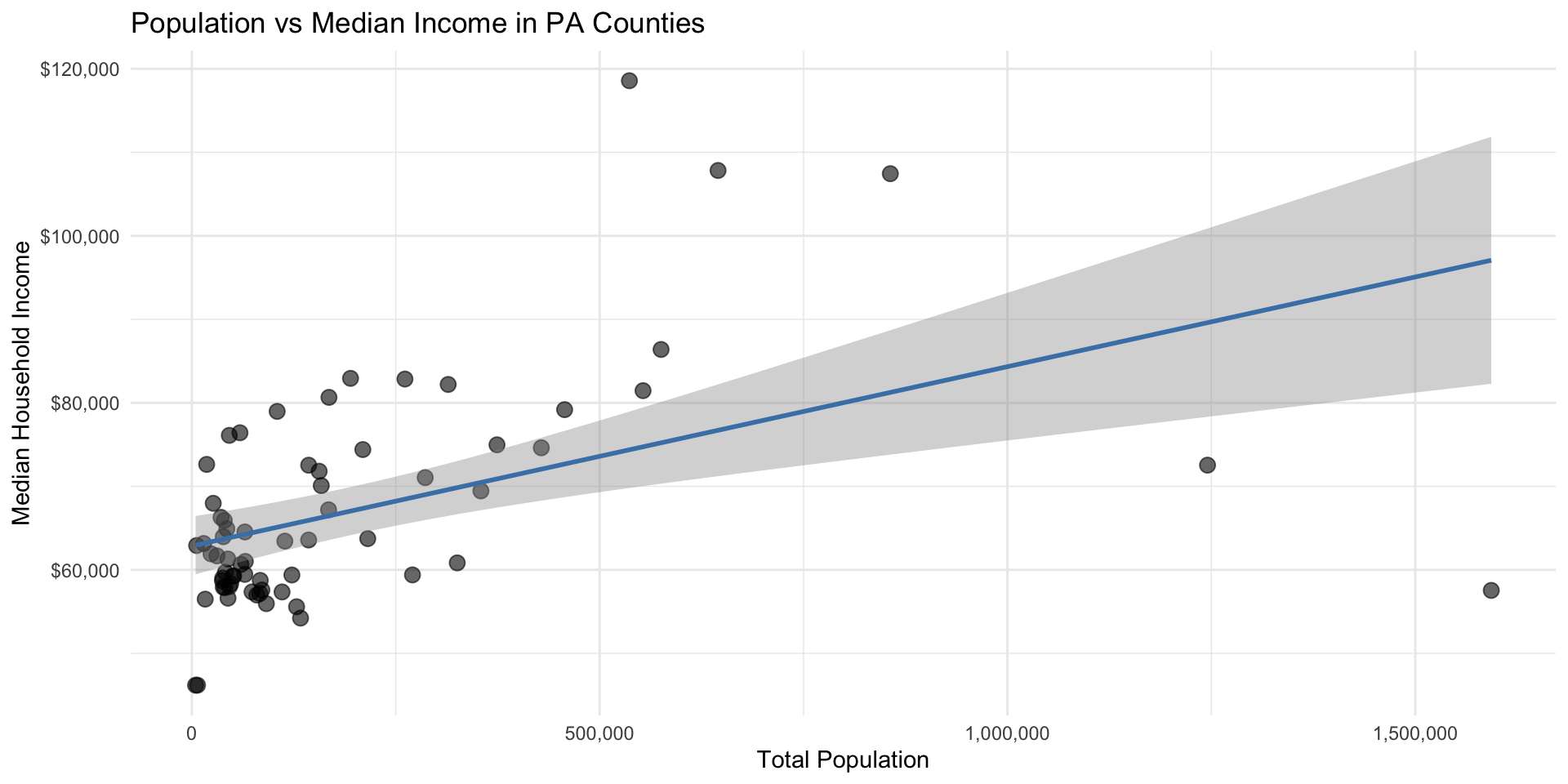
What Do We See?

Before fitting any model, discuss the visualization:

Generally positive relationship
Considerable scatter (not deterministic)
Most counties are small (clustered left)
One large county with surprisingly low income
Wider confidence band at higher populations

Question: What does this tell us about f(X)?

Fit the Model

model1 <- lm(median_incomeE ~ total_popE, data = pa_data)
summary(model1)


Call:
lm(formula = median_incomeE ~ total_popE, data = pa_data)

Residuals:
   Min     1Q Median     3Q    Max 
-39536  -6013  -1868   5075  44196 

Coefficients:
                Estimate   Std. Error t value             Pr(>|t|)    
(Intercept) 62855.819808  1760.477709  35.704 < 0.0000000000000002 ***
total_popE      0.021477     0.005192   4.137             0.000103 ***
---
Signif. codes:  0 '***' 0.001 '**' 0.01 '*' 0.05 '.' 0.1 ' ' 1

Residual standard error: 11820 on 65 degrees of freedom
Multiple R-squared:  0.2084,    Adjusted R-squared:  0.1962 
F-statistic: 17.11 on 1 and 65 DF,  p-value: 0.0001032

Interpreting Coefficients

Intercept (β₀) = $62,855

Expected income when population = 0
Not usually meaningful in practice

Slope (β₁) = $0.02

For each additional person, income increases by $0.02
More useful: For every 1,000 people, income increases by ~$20

Is this relationship real?

p-value < 0.001 → Very unlikely to see this if true β₁ = 0
We can reject the null hypothesis

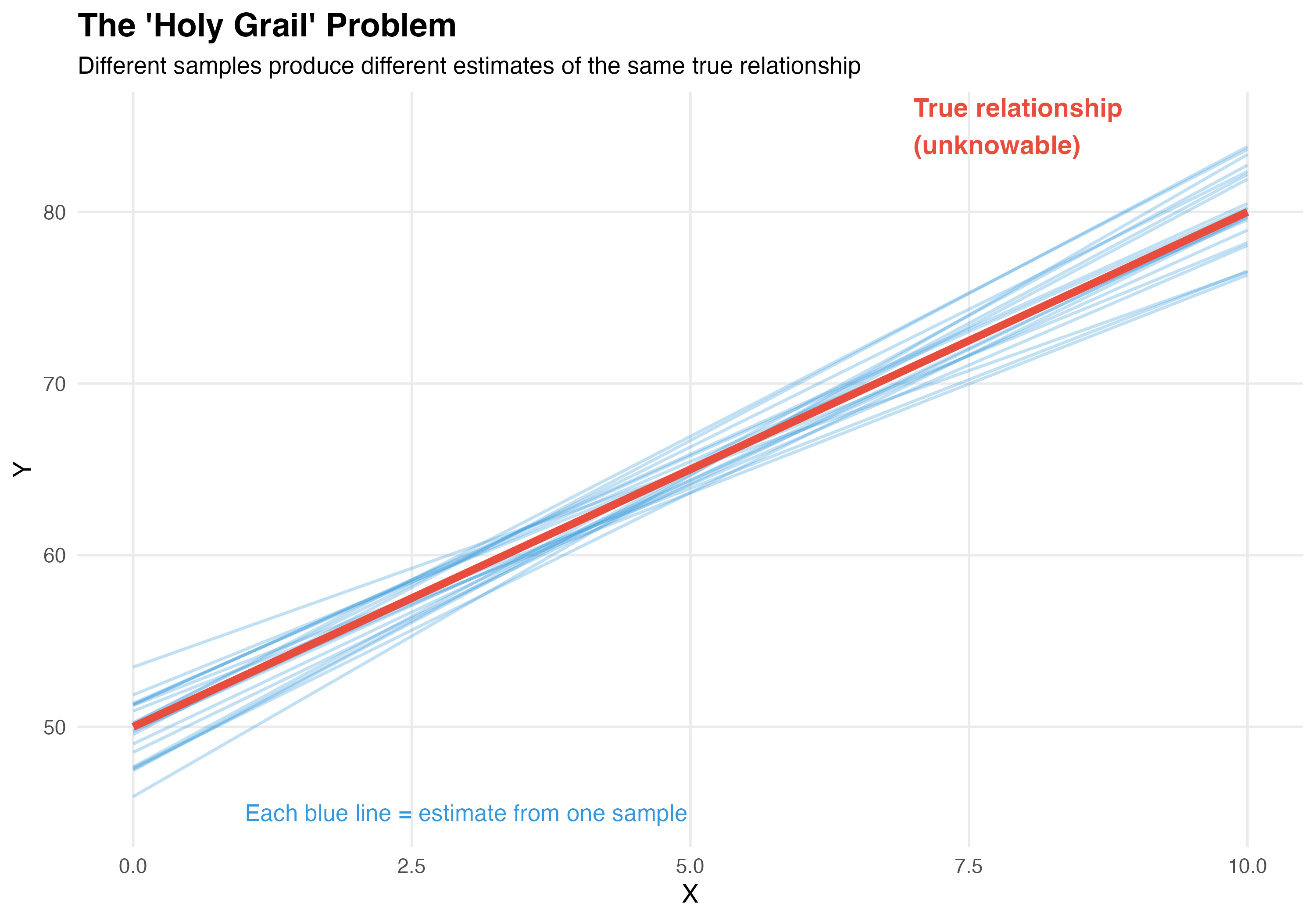
The “Holy Grail” Concept

Our estimates are just that: estimates of the true (unknown) parameters

Key insight:

Red line = true relationship (unknowable)
Blue line = our estimate from this sample
Different samples → slightly different blue lines
Standard errors quantify this uncertainty

Statistical Significance

The logic:

Null hypothesis (H₀): β₁ = 0 (no relationship)
Our estimate: β₁ = 0.02
Question: Could we get 0.02 just by chance if H₀ is true?

t-statistic: How many standard errors away from 0?

Bigger |t| = more confidence the relationship is real

p-value: Probability of seeing our estimate if H₀ is true

Small p → reject H₀, conclude relationship exists

Part 4: Model Evaluation

How Good is This Model?

Two key questions:

How well does it fit the data we used? (in-sample fit)
How well would it predict new data? (out-of-sample performance)

These are NOT the same thing!

In-Sample Fit: R²

R² = 0.208

“21% of variation in income is explained by population”

Is this good?

Depends on your goal!
For prediction: Moderate
For inference: Shows population matters, but other factors exist

R² alone doesn’t tell us if the model is trustworthy

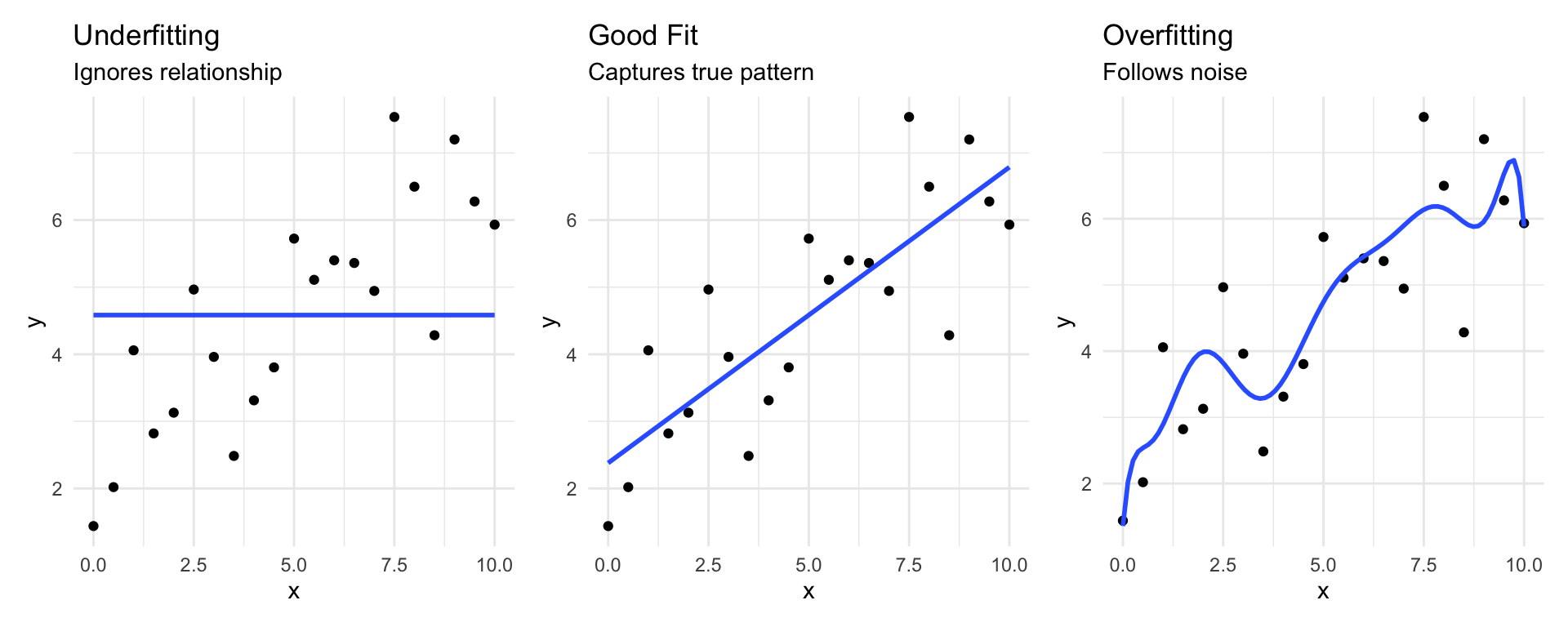
The Problem: Overfitting

Three scenarios:

Underfitting: Model too simple (high bias)
Good fit: Captures pattern without noise
Overfitting: Memorizes training data (high variance)

Overfitting in Regression

The danger: High R² doesn’t mean good predictions!

Train/Test Split

Solution: Hold out some data to test predictions

set.seed(123)
n <- nrow(pa_data)

# 70% training, 30% testing
train_indices <- sample(1:n, size = 0.7 * n)
train_data <- pa_data[train_indices, ]
test_data <- pa_data[-train_indices, ]

# Fit on training data only
model_train <- lm(median_incomeE ~ total_popE, data = train_data)

# Predict on test data
test_predictions <- predict(model_train, newdata = test_data)

Evaluate Predictions

# Calculate prediction error (RMSE)
rmse_test <- sqrt(mean((test_data$median_incomeE - test_predictions)^2))
rmse_train <- summary(model_train)$sigma

cat("Training RMSE:", round(rmse_train, 0), "\n")

Training RMSE: 12893

cat("Test RMSE:", round(rmse_test, 0), "\n")

Test RMSE: 9536

Interpreting RMSE

On new data (test set), our predictions are off by ~$9,500 on average. Is this level of error acceptable for policy decisions?

Cross-Validation

Better approach: Multiple train/test splits

Gives more stable estimate of true prediction performance

Cross-Validation in Action

library(caret)

# 10-fold cross-validation
train_control <- trainControl(method = "cv", number = 10)

cv_model <- train(median_incomeE ~ total_popE,
                  data = pa_data,
                  method = "lm",
                  trControl = train_control)

cv_model$results

  intercept     RMSE  Rsquared      MAE   RMSESD RsquaredSD    MAESD
1      TRUE 12577.76 0.5643826 8859.865 5609.002  0.2997098 2238.042

Key Metrics (Averaged Across 10 Folds)

RMSE: Typical prediction error (~$12,578)
R²: % of variation explained (0.564)
MAE: Average absolute error (~$8,860) - easier to interpret

Part 5: Checking Assumptions

When Can We Trust This Model?

Linear regression makes assumptions. If violated:

Coefficients may be biased
Standard errors wrong
Predictions unreliable

We must check diagnostics before trusting any model

Assumption 1: Linearity

What we assume: Relationship is actually linear

How to check: Residual plot

pa_data$residuals <- residuals(model1)
pa_data$fitted <- fitted(model1)

ggplot(pa_data, aes(x = fitted, y = residuals)) +
  geom_point() +
  geom_hline(yintercept = 0, color = "red", linetype = "dashed") +
  labs(title = "Residual Plot", x = "Fitted Values", y = "Residuals") +
  theme_minimal()

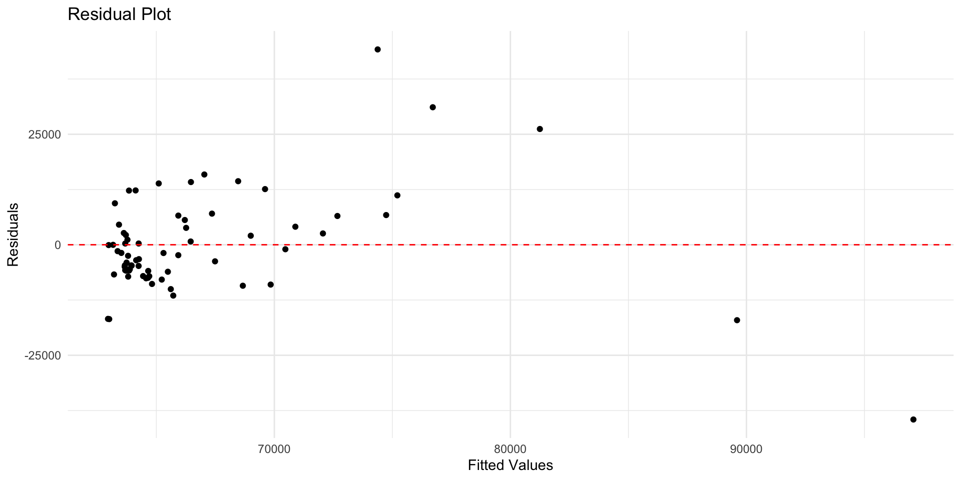
Reading Residual Plots

Good

Random scatter
Points around 0
Constant spread

Bad

Curved pattern
Model missing something
Predictions biased

Why This Matters for Prediction

Linearity violations hurt predictions, not just inference:

If the true relationship is curved and you fit a straight line, you’ll systematically underpredict in some regions and overpredict in others
Biased predictions in predictable ways (not random errors!)
Residual plots should show random scatter - any pattern means your model is missing something systematic

Assumption 2: Constant Variance

Heteroscedasticity: Variance changes across X

Impact: Standard errors are wrong → p-values misleading

What Heteroskedasticity Tells You

Often a symptom of model misspecification:

Model fits well for some values (e.g., small counties) but poorly for others (large counties)
May indicate missing variables that matter more at certain X values
Ask: “What’s different about observations with large residuals?”

Example: Population alone predicts income well in rural counties, but large urban counties need additional variables (education, industry) to predict accurately.

Heteroskedasticity Visualized

Key Insight: Adding the right predictor can fix heteroscedasticity

Formal Test: Breusch-Pagan

library(lmtest)
bptest(model1)


    studentized Breusch-Pagan test

data:  model1
BP = 27.481, df = 1, p-value = 0.0000001587

Interpretation:

p > 0.05: Constant variance assumption OK
p < 0.05: Evidence of heteroscedasticity

If detected, solutions:

Transform Y (try log(income))
Robust standard errors
Add missing variables
Accept it (point predictions still OK for prediction goals)

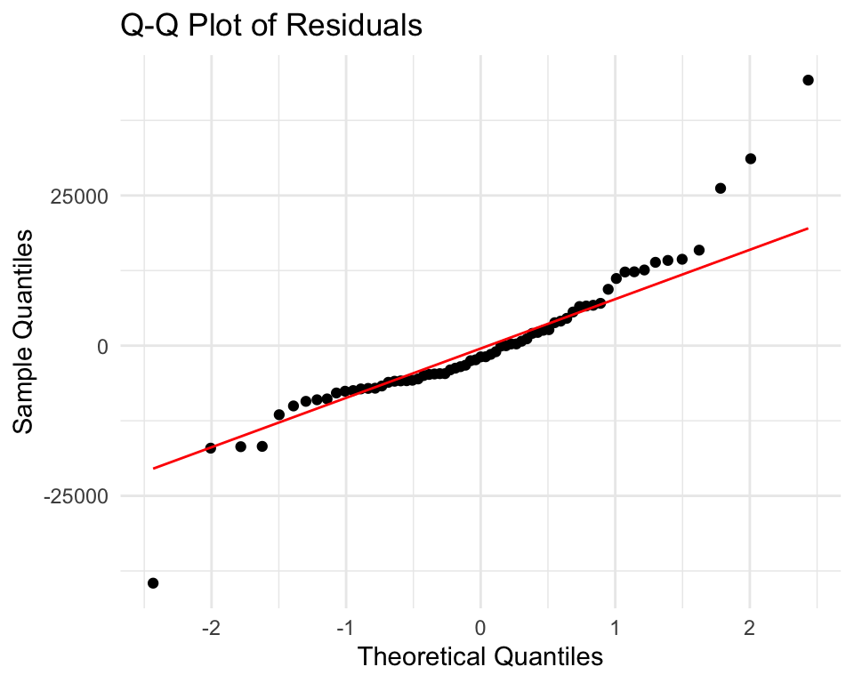
Assumption: Normality of Residuals

What we assume: Residuals are normally distributed

Why it matters:

Less critical for point predictions (unbiased regardless)
Important for confidence intervals and prediction intervals
Needed for valid hypothesis tests (t-tests, F-tests)

Q-Q Plot

Assumption 3: No Multicollinearity

For multiple regression: Predictors shouldn’t be too correlated

library(car)
vif(model1)  # Variance Inflation Factor

# Rule of thumb: VIF > 10 suggests problems
# Not relevant with only 1 predictor!

Why it matters: Coefficients become unstable, hard to interpret

Assumption 4: No Influential Outliers

Not all outliers are problems - only those with high leverage AND large residuals

Visual Diagnostic

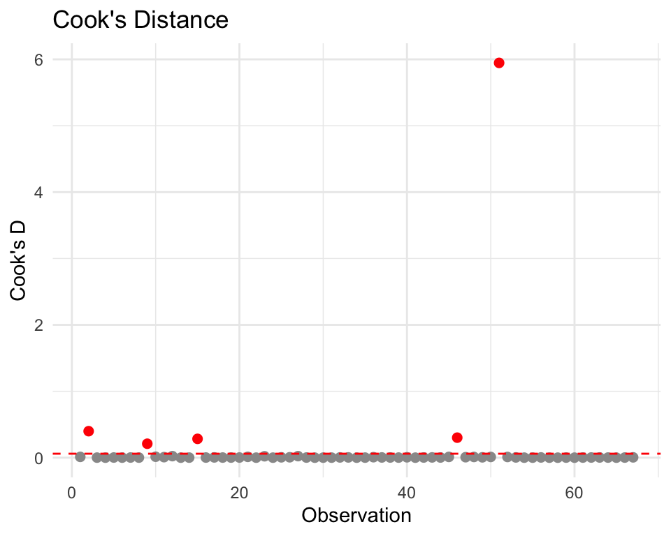
Identify Influential Points

# A tibble: 2 × 4
  NAME                              total_popE median_incomeE cooks_d
  <chr>                                  <dbl>          <dbl>   <dbl>
1 Philadelphia County, Pennsylvania    1593208          57537   5.95 
2 Allegheny County, Pennsylvania       1245310          72537   0.399

Interpretation:

Cook’s D > 4/n = potentially influential
High leverage + large residual = pulls regression line

What To Do With Influential Points

Investigation Strategy

Investigate: Why is this observation unusual? (data error? truly unique?)
Report: Always note influential observations in your analysis
Sensitivity check: Refit model without them - do conclusions change?
Don’t automatically remove: They might represent real, important cases

For policy: An influential county might need special attention, not exclusion!

Connection to Algorithmic Bias

High-influence observations in demographic could represent marginalized communities or unique populations. Automatically removing them can erase important populations from analysis and lead to biased policy decisions.

Always investigate before removing!

Part 6: Improving the Model

Adding More Predictors

Maybe population alone isn’t enough:


Call:
lm(formula = median_incomeE ~ total_popE + percent_collegeE + 
    poverty_rateE, data = pa_data_full)

Residuals:
   Min     1Q Median     3Q    Max 
-32939  -4473  -1098   3861  27672 

Coefficients:
                    Estimate  Std. Error t value             Pr(>|t|)    
(Intercept)      60893.86796  1589.24122  38.316 < 0.0000000000000002 ***
total_popE           0.06657     0.03356   1.984               0.0517 .  
percent_collegeE     0.04710     0.14916   0.316               0.7532    
poverty_rateE       -0.36503     0.07749  -4.711             0.000014 ***
---
Signif. codes:  0 '***' 0.001 '**' 0.01 '*' 0.05 '.' 0.1 ' ' 1

Residual standard error: 8610 on 63 degrees of freedom
Multiple R-squared:  0.5931,    Adjusted R-squared:  0.5738 
F-statistic: 30.61 on 3 and 63 DF,  p-value: 0.000000000002485

Log Transformations

If relationship is curved, try transforming:

# Compare linear vs log
model_linear <- lm(median_incomeE ~ total_popE, data = pa_data)
model_log <- lm(median_incomeE ~ log(total_popE), data = pa_data)

summary(model_log)


Call:
lm(formula = median_incomeE ~ log(total_popE), data = pa_data)

Residuals:
   Min     1Q Median     3Q    Max 
-27231  -5780  -2118   3953  40638 

Coefficients:
                Estimate Std. Error t value   Pr(>|t|)    
(Intercept)        -4867      12374  -0.393      0.695    
log(total_popE)     6276       1074   5.842 0.00000018 ***
---
Signif. codes:  0 '***' 0.001 '**' 0.01 '*' 0.05 '.' 0.1 ' ' 1

Residual standard error: 10760 on 65 degrees of freedom
Multiple R-squared:  0.3443,    Adjusted R-squared:  0.3342 
F-statistic: 34.13 on 1 and 65 DF,  p-value: 0.0000001805

# Check which residual plot looks better

Interpretation changes: Log models show percentage relationships

Categorical Variables

# Create metro/non-metro indicator
pa_data <- pa_data %>%
  mutate(metro = ifelse(total_popE > 500000, 1, 0))

model3 <- lm(median_incomeE ~ total_popE + metro, data = pa_data)
summary(model3)


Call:
lm(formula = median_incomeE ~ total_popE + metro, data = pa_data)

Residuals:
   Min     1Q Median     3Q    Max 
-28824  -6732  -2885   7672  26622 

Coefficients:
                Estimate   Std. Error t value             Pr(>|t|)    
(Intercept) 64924.857892  1659.821786  39.116 < 0.0000000000000002 ***
total_popE     -0.005290     0.008047  -0.657             0.513257    
metro       29865.529225  7319.309190   4.080             0.000127 ***
---
Signif. codes:  0 '***' 0.001 '**' 0.01 '*' 0.05 '.' 0.1 ' ' 1

Residual standard error: 10610 on 64 degrees of freedom
Multiple R-squared:  0.3718,    Adjusted R-squared:  0.3522 
F-statistic: 18.94 on 2 and 64 DF,  p-value: 0.0000003456

R creates dummy variables automatically

Summary: The Regression Workflow

Understand the framework: What’s f? What’s the goal?
Visualize first: Does a linear model make sense?
Fit the model: Estimate coefficients
Evaluate performance: Train/test split, cross-validation
Check assumptions: Residual plots, VIF, outliers
Improve if needed: Transformations, more variables
Consider ethics: Who could be harmed by this model?

Key Takeaways

Statistical Learning:

We’re estimating f(X), the systematic relationship
Parametric methods assume a form (we chose linear)

Two purposes:

Inference: understand relationships
Prediction: forecast new values

Model evaluation:

In-sample fit ≠ out-of-sample performance
Beware overfitting!

Diagnostics matter:

Always check assumptions
Plots reveal what R² hides

🏆 Learning- Focused In-Class Challenge:

Best Predictive Model Competition

The Task

Predict median home value (B25077_001) for PA counties using any combination of predictors

Build the model with lowest 10-fold cross-validated RMSE

Available Predictors

challenge_data <- get_acs(
  geography = "county",
  state = "PA",
  variables = c(
    home_value = "B25077_001",      # YOUR TARGET
    total_pop = "B01003_001",       # Total population
    median_income = "B19013_001",   # Median household income
    median_age = "B01002_001",      # Median age
    percent_college = "B15003_022", # Bachelor's degree or higher
    median_rent = "B25058_001",     # Median rent
    poverty_rate = "B17001_002"     # Population in poverty
  ),
  year = 2022,
  output = "wide"
)

Rules & Strategy

You can:

Use any combination of predictors (time permitting, you can fetch more)
Try log transformations: log(total_popE)
Engineer new categorical features
Remove influential outliers (but document which!)

You must:

Use 10-fold cross-validation to report final RMSE
Do a full diagnostic check (residual plot, Cook’s D, or Breusch-Pagan)
Be ready to explain your model in 2 minutes

Hints

Start simple (one predictor), check diagnostics
Income and rent are probably highly correlated (multicollinearity!)
Try log transformation if relationship looks curved
Don’t forget to remove NAs: na.omit(challenge_data)