Spatial Machine Learning & Advanced Regression

Week 6: MUSA 5080

Dr. Elizabeth Delmelle

2025-10-14

Today’s Journey

What We’ll Cover

Warm-Up: Build a Baseline Model

Quick review of Week 5 regression
Create simple structural model
Identify its limitations

Part 1: Expanding Your Toolkit

Categorical variables
Interactions
Polynomial terms

Part 2: Why Space Matters

Hedonic model framework
Tobler’s First Law
Spatial autocorrelation

Part 3: Creating Spatial Features

Buffer aggregation
k-Nearest Neighbors
Distance to amenities

Part 4: Fixed Effects

Warm-Up: Build a Baseline Model

Let’s Build Something Simple Together

We’ll start by creating a basic model using only structural features - this will be our baseline to improve upon today.

# Load packages and data
library(tidyverse)
library(sf)
library(here)

# Load Boston housing data
boston <- read_csv(here("data/boston.csv"))

# Quick look at the data
glimpse(boston)

Rows: 1,485
Columns: 24
$ ...1       <dbl> 1, 2, 3, 4, 5, 6, 7, 8, 9, 10, 11, 12, 13, 14, 15, 16, 17, …
$ Parcel_No  <dbl> 100032000, 100058000, 100073000, 100112000, 100137000, 1001…
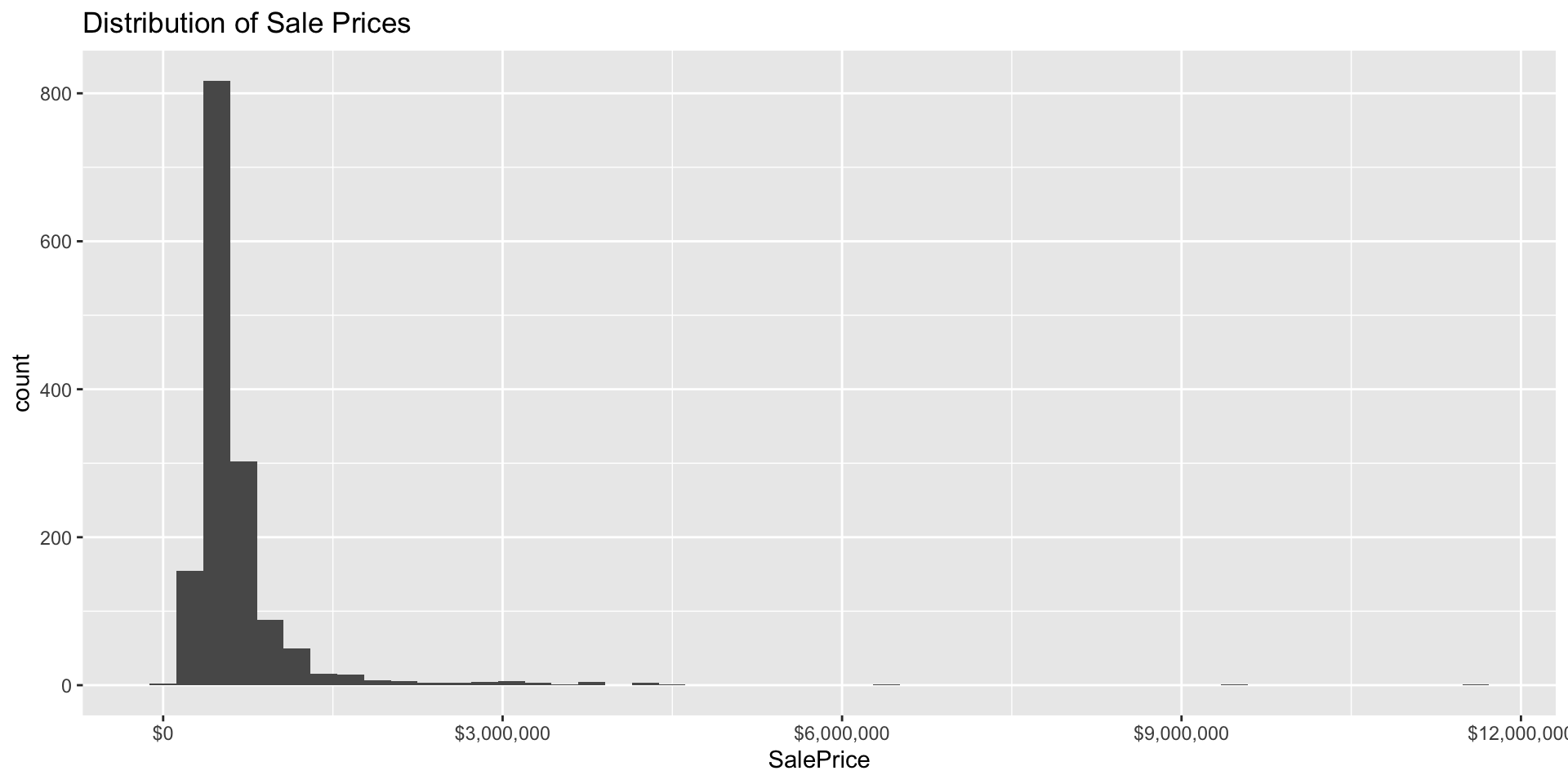
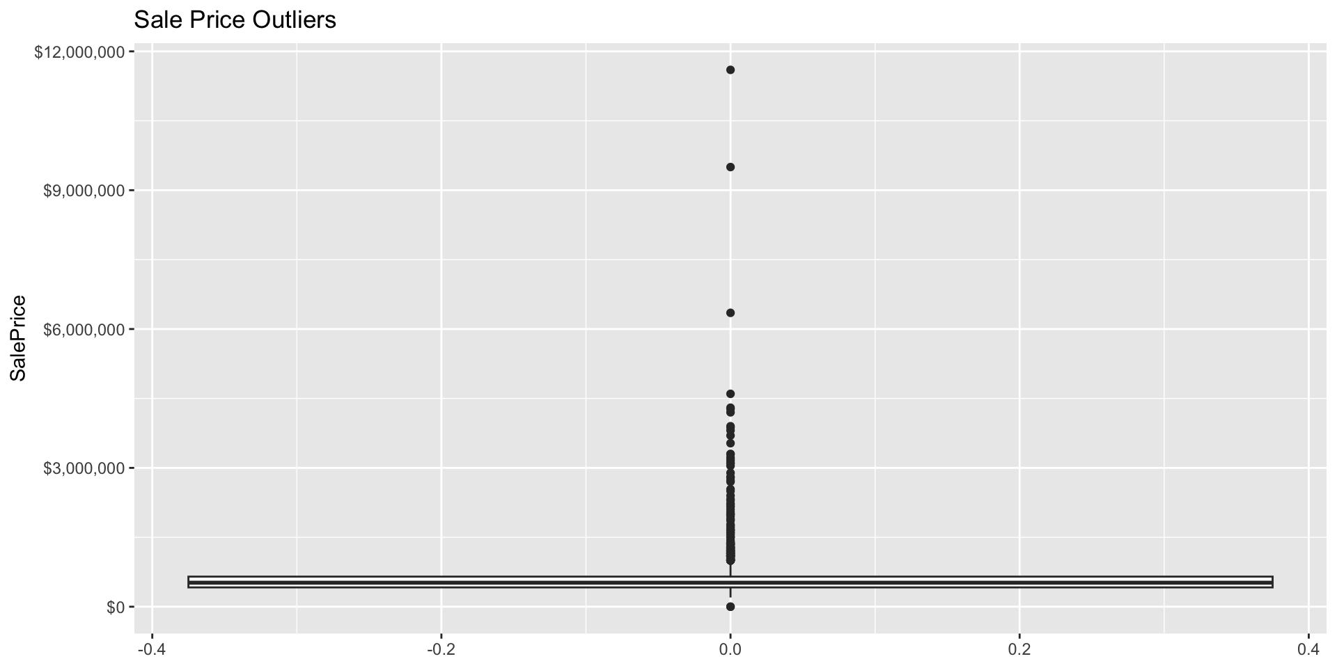
$ SalePrice  <dbl> 450000, 600000, 450000, 670000, 260000, 355000, 665000, 355…
$ PricePerSq <dbl> 228.89, 164.34, 105.98, 291.94, 217.21, 190.96, 227.35, 120…
$ LivingArea <dbl> 1966, 3840, 4246, 2295, 1197, 1859, 2925, 2904, 892, 1916, …
$ Style      <chr> "Conventional", "Semi?Det", "Decker", "Row\xa0End", "Coloni…
$ GROSS_AREA <dbl> 3111, 5603, 6010, 3482, 1785, 2198, 4341, 3892, 1658, 3318,…
$ NUM_FLOORS <dbl> 2.0, 3.0, 3.0, 3.0, 2.0, 1.5, 3.0, 3.0, 2.0, 2.0, 1.5, 2.0,…
$ R_BDRMS    <dbl> 4, 8, 9, 6, 2, 3, 8, 6, 2, 2, 4, 3, 3, 3, 6, 8, 4, 4, 3, 2,…
$ R_FULL_BTH <dbl> 2, 3, 3, 3, 1, 3, 3, 3, 1, 2, 2, 3, 1, 1, 3, 3, 2, 3, 1, 2,…
$ R_HALF_BTH <dbl> 0, 0, 0, 0, 1, 0, 0, 0, 0, 0, 0, 0, 0, 1, 0, 0, 0, 1, 0, 0,…
$ R_KITCH    <dbl> 2, 3, 3, 3, 1, 2, 3, 3, 1, 2, 2, 3, 1, 1, 3, 3, 2, 3, 2, 2,…
$ R_AC       <chr> "N", "N", "N", "N", "N", "N", "N", "N", "N", "N", "N", "N",…
$ R_FPLACE   <dbl> 0, 0, 0, 0, 0, 0, 0, 0, 0, 0, 0, 0, 0, 0, 0, 0, 0, 0, 0, 0,…
$ LU         <chr> "R2", "R3", "R3", "R3", "R1", "R2", "R3", "E", "R1", "R2", …
$ OWN_OCC    <chr> "Y", "N", "Y", "N", "N", "N", "N", "N", "N", "Y", "N", "N",…
$ R_BLDG_STY <chr> "CV", "SD", "DK", "RE", "CL", "CV", "DK", "DK", "RE", "TF",…
$ R_ROOF_TYP <chr> "H", "F", "F", "F", "F", "G", "F", "F", "G", "F", "G", "F",…
$ R_EXT_FIN  <chr> "M", "B", "M", "M", "P", "M", "M", "A", "A", "M", "W", "W",…
$ R_TOTAL_RM <dbl> 10, 17, 20, 14, 5, 8, 14, 14, 4, 9, 7, 7, 5, 5, 15, 14, 11,…
$ R_HEAT_TYP <chr> "W", "W", "W", "W", "E", "E", "W", "W", "W", "W", "W", "W",…
$ YR_BUILT   <dbl> 1900, 1910, 1910, 1905, 1860, 1905, 1900, 1890, 1900, 1900,…
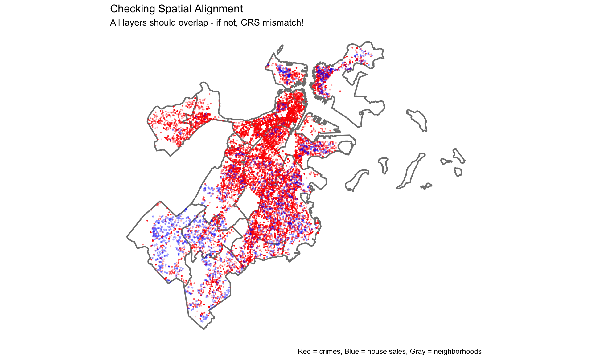
$ Latitude   <dbl> 42.37963, 42.37877, 42.37940, 42.38014, 42.37967, 42.37953,…
$ Longitude  <dbl> -71.03076, -71.02943, -71.02846, -71.02859, -71.02903, -71.…

# Simple model: Predict price from living area
baseline_model <- lm(SalePrice ~ LivingArea, data = boston)
summary(baseline_model)


Call:
lm(formula = SalePrice ~ LivingArea, data = boston)

Residuals:
    Min      1Q  Median      3Q     Max 
-855962 -219491  -68291   55248 9296561 

Coefficients:
             Estimate Std. Error t value Pr(>|t|)    
(Intercept) 157968.32   35855.59   4.406 1.13e-05 ***
LivingArea     216.54      14.47  14.969  < 2e-16 ***
---
Signif. codes:  0 '***' 0.001 '**' 0.01 '*' 0.05 '.' 0.1 ' ' 1

Residual standard error: 563800 on 1483 degrees of freedom
Multiple R-squared:  0.1313,    Adjusted R-squared:  0.1307 
F-statistic: 224.1 on 1 and 1483 DF,  p-value: < 2.2e-16

What Does This Model Tell Us?


Call:
lm(formula = SalePrice ~ LivingArea, data = boston)

Residuals:
    Min      1Q  Median      3Q     Max 
-855962 -219491  -68291   55248 9296561 

Coefficients:
             Estimate Std. Error t value Pr(>|t|)    
(Intercept) 157968.32   35855.59   4.406 1.13e-05 ***
LivingArea     216.54      14.47  14.969  < 2e-16 ***
---
Signif. codes:  0 '***' 0.001 '**' 0.01 '*' 0.05 '.' 0.1 ' ' 1

Residual standard error: 563800 on 1483 degrees of freedom
Multiple R-squared:  0.1313,    Adjusted R-squared:  0.1307 
F-statistic: 224.1 on 1 and 1483 DF,  p-value: < 2.2e-16

[1] 0.1312636

Interpreting Our Baseline

Expected Output:

Variable	Coefficient	Std. Error	t-value	p-value
Intercept	157968.32	35855.59	4.406	<0.001
LivingArea	216.54	14.47	14.969	<0.001

What this means:

Base price (0 sq ft) ≈ 157968.32
Each additional square foot adds ~216 to price
Relationship is statistically significant (p < 0.001)
But R² is only 0.13 (13% of variation explained)

The Problem

MOST of the variation in house prices is still unexplained!

What are we missing? 🤔

Limitations of This Model

What’s Missing?

What does this model ignore?
- Location! (North End vs. Roxbury vs. Back Bay)
- Proximity to downtown, waterfront, parks
- Nearby crime levels
- School quality
- Neighborhood characteristics
Why might it fail?
- 1,000 sq ft in Back Bay ≠ 1,000 sq ft in Roxbury
- Same house, different locations → vastly different prices
- “Location, location, location!”
How could we improve it?
- Add spatial features (crime nearby, distance to amenities)
- Control for neighborhood (fixed effects)
- Include interactions (does size matter more in wealthy areas?)

This is exactly where spatial features come in!

Let’s Add One More Feature

# Add number of bathrooms
better_model <- lm(SalePrice ~ LivingArea + R_FULL_BTH, data = boston)
summary(better_model)


Call:
lm(formula = SalePrice ~ LivingArea + R_FULL_BTH, data = boston)

Residuals:
    Min      1Q  Median      3Q     Max 
-783019 -230756  -65737   75367 9193133 

Coefficients:
             Estimate Std. Error t value Pr(>|t|)    
(Intercept) 107683.96   37340.88   2.884  0.00399 ** 
LivingArea     145.68      21.33   6.828 1.25e-11 ***
R_FULL_BTH  106978.13   23800.30   4.495 7.50e-06 ***
---
Signif. codes:  0 '***' 0.001 '**' 0.01 '*' 0.05 '.' 0.1 ' ' 1

Residual standard error: 560200 on 1482 degrees of freedom
Multiple R-squared:  0.1429,    Adjusted R-squared:  0.1418 
F-statistic: 123.6 on 2 and 1482 DF,  p-value: < 2.2e-16

# Compare models
cat("Baseline R²:", summary(baseline_model)$r.squared, "\n")

Baseline R²: 0.1312636

cat("With bathrooms R²:", summary(better_model)$r.squared, "\n")

With bathrooms R²: 0.1429474

R² improves a smidge… but still missing location!

Today’s Goal

By the end of class, you’ll build models that: - Incorporate spatial relationships - Account for neighborhood effects
- Achieve much better prediction accuracy - Help you understand what drives housing prices

Converting to Spatial Data

Step 1: Make your data spatial

library(sf)

# Convert boston data to sf object
boston.sf <- boston %>%
  st_as_sf(coords = c("Longitude", "Latitude"), crs = 4326) %>%
  st_transform('ESRI:102286')  # MA State Plane (feet)

# Check it worked
head(boston.sf)

Simple feature collection with 6 features and 22 fields
Geometry type: POINT
Dimension:     XY
Bounding box:  xmin: 238643.6 ymin: 903246 xmax: 238833.2 ymax: 903399.5
Projected CRS: NAD_1983_HARN_StatePlane_Massachusetts_Mainland_FIPS_2001
# A tibble: 6 × 23
   ...1 Parcel_No SalePrice PricePerSq LivingArea Style    GROSS_AREA NUM_FLOORS
  <dbl>     <dbl>     <dbl>      <dbl>      <dbl> <chr>         <dbl>      <dbl>
1     1 100032000    450000       229.       1966 "Conven…       3111        2  
2     2 100058000    600000       164.       3840 "Semi?D…       5603        3  
3     3 100073000    450000       106.       4246 "Decker"       6010        3  
4     4 100112000    670000       292.       2295 "Row\xa…       3482        3  
5     5 100137000    260000       217.       1197 "Coloni…       1785        2  
6     6 100138000    355000       191.       1859 "Conven…       2198        1.5
# ℹ 15 more variables: R_BDRMS <dbl>, R_FULL_BTH <dbl>, R_HALF_BTH <dbl>,
#   R_KITCH <dbl>, R_AC <chr>, R_FPLACE <dbl>, LU <chr>, OWN_OCC <chr>,
#   R_BLDG_STY <chr>, R_ROOF_TYP <chr>, R_EXT_FIN <chr>, R_TOTAL_RM <dbl>,
#   R_HEAT_TYP <chr>, YR_BUILT <dbl>, geometry <POINT [m]>

class(boston.sf)  # Should show "sf" and "data.frame"

[1] "sf"         "tbl_df"     "tbl"        "data.frame"

Why transform CRS?

4326 = WGS84 (lat/lon in degrees) - fine for display
ESRI:102286 = MA State Plane (feet) - good for distance calculations

Step 2: Spatial Join with Neighborhoods

# Load neighborhood boundaries
nhoods <- read_sf(here("data/BPDA_Neighborhood_Boundaries.geojson")) %>%
  st_transform('ESRI:102286')  # Match CRS!

# Check the neighborhoods
head(nhoods)

Simple feature collection with 6 features and 7 fields
Geometry type: MULTIPOLYGON
Dimension:     XY
Bounding box:  xmin: 229049.1 ymin: 890856 xmax: 236590.9 ymax: 900302.5
Projected CRS: NAD_1983_HARN_StatePlane_Massachusetts_Mainland_FIPS_2001
# A tibble: 6 × 8
  sqmiles name         neighborhood_id  acres SHAPE__Length objectid SHAPE__Area
    <dbl> <chr>        <chr>            <dbl>         <dbl>    <int>       <dbl>
1    2.51 Roslindale   15              1606.         53564.       53   69938273.
2    3.94 Jamaica Pla… 11              2519.         56350.       54  109737890.
3    0.55 Mission Hill 13               351.         17919.       55   15283120.
4    0.29 Longwood     28               189.         11909.       56    8215904.
5    0.04 Bay Village  33                26.5         4651.       57    1156071.
6    0.02 Leather Dis… 27                15.6         3237.       58     681272.
# ℹ 1 more variable: geometry <MULTIPOLYGON [m]>

nrow(nhoods)  # How many neighborhoods?

[1] 26

# Spatial join: Assign each house to its neighborhood
boston.sf <- boston.sf %>%
  st_join(nhoods, join = st_intersects)

# Check results
boston.sf %>%
  st_drop_geometry() %>%
  count(name) %>%
  arrange(desc(n))

# A tibble: 19 × 2
   name              n
   <chr>         <int>
 1 Dorchester      344
 2 West Roxbury    242
 3 Hyde Park       152
 4 East Boston     149
 5 Roslindale      142
 6 Jamaica Plain   113
 7 South Boston     80
 8 Charlestown      65
 9 Mattapan         65
10 Roxbury          63
11 South End        20
12 Beacon Hill      17
13 Mission Hill     14
14 Allston           6
15 Brighton          6
16 Back Bay          3
17 Fenway            2
18 Bay Village       1
19 Downtown          1

What just happened?

st_join() found which neighborhood polygon contains each house point!

Visualize: Prices by Neighborhood

The Spatial Pattern is Clear!

# Which neighborhoods are most expensive?
price_by_nhood %>%
  arrange(desc(median_price)) %>%
  head(5)

# A tibble: 5 × 3
  name        median_price n_sales
  <chr>              <dbl>   <int>
1 Back Bay         9500000       3
2 Beacon Hill      2892750      17
3 South End        2797500      20
4 Bay Village      2300000       1
5 Fenway           2112500       2

# Which have most sales?
price_by_nhood %>%
  arrange(desc(n_sales)) %>%
  head(5)

# A tibble: 5 × 3
  name         median_price n_sales
  <chr>               <dbl>   <int>
1 Dorchester         511250     344
2 West Roxbury       503750     242
3 Hyde Park          390000     152
4 East Boston        463000     149
5 Roslindale         489500     142

Discussion Question

Why do you think certain neighborhoods command higher prices? - Proximity to downtown? - Historical character? - School quality? - Safety? - All of the above?

This is why we need spatial features and neighborhood controls!

Part 1: Expanding Your Regression Toolkit

Beyond Continuous Variables

✅ Continuous Variables

Square footage
Age of house
Income levels
Distance to downtown

🏷️ Categorical Variables

Neighborhood
School district
Building type
Has garage? (Yes/No)

Dummy Variables

Our Boston Data: `name` variable from spatial join

Neighborhoods in our dataset (showing just a few):

# A tibble: 10 × 2
   name              n
   <chr>         <int>
 1 Dorchester      344
 2 West Roxbury    242
 3 Hyde Park       152
 4 East Boston     149
 5 Roslindale      142
 6 Jamaica Plain   113
 7 South Boston     80
 8 Charlestown      65
 9 Mattapan         65
10 Roxbury          63

How R Handles This

When you include name in a model, R automatically creates binary indicators:

Back_Bay: 1 if Back Bay, 0 otherwise
Beacon_Hill: 1 if Beacon Hill, 0 otherwise
Charlestown: 1 if Charlestown, 0 otherwise
…and so on for all neighborhoods

⚠️ The (n-1) Rule

One neighborhood is automatically chosen as the reference category (omitted)!

R picks the first alphabetically unless you specify otherwise.

Add Dummy (Categorical) Variables to the Model

# Ensure name is a factor
boston.sf <- boston.sf %>%
  mutate(name = as.factor(name))

# Check which is reference (first alphabetically)
levels(boston.sf$name)[1]

[1] "Allston"

# Fit model with neighborhood fixed effects
model_neighborhoods <- lm(SalePrice ~ LivingArea + name, 
                          data = boston.sf)

# Show just first 10 coefficients
summary(model_neighborhoods)$coef[1:10, ]

                    Estimate   Std. Error    t value      Pr(>|t|)
(Intercept)      704306.0751 9.022210e+04  7.8063584  1.112892e-14
LivingArea          138.3206 6.468186e+00 21.3847638  1.605175e-88
nameBack Bay    7525585.0560 1.533714e+05 49.0677253 1.522921e-311
nameBay Village 1284057.5326 2.320256e+05  5.5341206  3.700442e-08
nameBeacon Hill 1767805.2297 1.020211e+05 17.3278366  2.465874e-61
nameBrighton    -168941.2113 1.239972e+05 -1.3624597  1.732623e-01
nameCharlestown   -2556.8667 9.208989e+04 -0.0277649  9.778534e-01
nameDorchester  -576819.4858 8.846990e+04 -6.5199517  9.653393e-11
nameDowntown      58553.1237 2.322150e+05  0.2521505  8.009601e-01
nameEast Boston -534060.4110 8.962950e+04 -5.9585340  3.182615e-09

Interpreting Neighborhood Dummy Variables

Variable	Coefficient	p-value
Intercept (Allston)	$649,635	< 0.001***
Living Area (per sq ft)	$114	< 0.001***
Back Bay	$7,561,273	< 0.001***
Beacon Hill	$1,780,861	< 0.001***
Charlestown	$22,575	0.806
Dorchester	-$540,267	< 0.001***
East Boston	-$515,990	< 0.001***
Roxbury	-$566,534	< 0.001***

How to Read This Table

Reference Category: Allston (automatically chosen - alphabetically first)

Structural Variables:

Living Area: Each additional sq ft adds this amount (same for all neighborhoods)
Bedrooms: Effect of one more full bathroom (same for all neighborhoods)

Neighborhood Dummies:

Positive coefficient = This neighborhood is MORE expensive than Allston
Negative coefficient = This neighborhood is LESS expensive than Allston
All else equal (same size, same bathrooms)

Concrete Example: Comparing Two Houses

Using our model, let’s compare identical houses in different neighborhoods:

House A: Back Bay

Living Area: 1,500 sq ft
Baths: 2
Neighborhood: Back Bay

Predicted Price:

           1 
"$8,458,873"

House B: Roxbury

Living Area: 1,500 sq ft
Baths: 2
Neighborhood: Roxbury

Predicted Price:

         1 
"$331,066"

Important

The Neighborhood Effect Price Difference

           1 
"$8,127,807"

Same house, different location = huge price difference! This is what the neighborhood dummies capture.

Interaction Effects: When Relationships Depend

The Question

Does the effect of one variable depend on the level of another variable?

Example Scenarios

Housing: Does square footage matter more in wealthy neighborhoods?
Education: Do tutoring effects vary by initial skill level?
Public Health: Do pollution effects differ by age?

Mathematical Form

SalePrice = β₀ + β₁(LivingArea) + β₂(WealthyNeighborhood) + β₃(LivingArea × WealthyNeighborhood) + ε

Today’s example: Is the value of square footage the same across all Boston neighborhoods?

Theory: Luxury Premium Hypothesis

🏛️ In Wealthy Neighborhoods

(Back Bay, Beacon Hill, South End)

High-end buyers pay premium for space
Luxury finishes, location prestige
Each sq ft adds substantial value
Steep slope

Hypothesis: $300+ per sq ft

🏘️ In Working-Class Neighborhoods

(Dorchester, Mattapan, East Boston)

Buyers value function over luxury
More price-sensitive market
Space matters, but less premium
Flatter slope

Hypothesis: $100-150 per sq ft

The Key Question

If we assume one slope for all neighborhoods, are we misunderstanding the market?

Create the Neighborhood Categories

# Define wealthy neighborhoods based on median prices
wealthy_hoods <- c("Back Bay", "Beacon Hill", "South End", "Bay Village")

# Create binary indicator
boston.sf <- boston.sf %>%
  mutate(
    wealthy_neighborhood = ifelse(name %in% wealthy_hoods, "Wealthy", "Not Wealthy"),
    wealthy_neighborhood = as.factor(wealthy_neighborhood)
  )

# Check the split
boston.sf %>%
  st_drop_geometry() %>%
  count(wealthy_neighborhood)

# A tibble: 2 × 2
  wealthy_neighborhood     n
  <fct>                <int>
1 Not Wealthy           1444
2 Wealthy                 41

Model 1: No Interaction (Parallel Slopes)

# Model assumes same slope everywhere
model_no_interact <- lm(SalePrice ~ LivingArea + wealthy_neighborhood, 
                        data = boston.sf)

summary(model_no_interact)$coef

                                Estimate   Std. Error   t value      Pr(>|t|)
(Intercept)                  213842.7642 23893.619394  8.949785  1.039392e-18
LivingArea                      160.2357     9.713346 16.496442  2.936087e-56
wealthy_neighborhoodWealthy 2591012.0471 59958.794614 43.213211 1.103579e-264

Warning

What This Assumes

Living area has the same effect in all neighborhoods Only the intercept differs (wealthy areas start higher) Parallel lines on a plot

Model 2: With Interaction (Different Slopes)

# Model allows different slopes
model_interact <- lm(SalePrice ~ LivingArea * wealthy_neighborhood, 
                     data = boston.sf)

summary(model_interact)$coef

                                            Estimate   Std. Error   t value
(Intercept)                             358542.41696 1.863997e+04 19.235144
LivingArea                                  95.63947 7.620382e+00 12.550483
wealthy_neighborhoodWealthy            -377937.38372 1.005554e+05 -3.758498
LivingArea:wealthy_neighborhoodWealthy     985.12500 2.975904e+01 33.103383
                                            Pr(>|t|)
(Intercept)                             8.875710e-74
LivingArea                              2.079700e-34
wealthy_neighborhoodWealthy             1.775774e-04
LivingArea:wealthy_neighborhoodWealthy 2.445570e-180

Important

What This Allows

Living area can have different effects in different neighborhoods Both intercept AND slope differ Non-parallel lines on a plot

Interpreting the Interaction Coefficients

Term	Coefficient	t-value	Sig
Intercept (Not Wealthy)	$358,542	19.235	***
Living Area (Not Wealthy)	$96	12.550	***
Wealthy Neighborhood Premium	-$377,937	-3.758	***
Extra $/sq ft in Wealthy Areas	$985	33.103	***

We get the un-intuitive negative premium here because that is an intercept adjustment (applies at 0 sqft). The slope difference (+985sq/ft) is huge - we can calculate when wealthy areas become more expensive (at what sq ft) = 384.

Breaking Down the Coefficients

🏘️ Not Wealthy Areas Equation: Price = $358,542 + $96 × LivingArea Interpretation:

Base price: $358,542 Each sq ft adds: $96

🏛️ Wealthy Areas Equation: Price = -$19,395 + $1,081 × LivingArea Interpretation:

Base price: -$19,395 Each sq ft adds: $1,081

Important

The Interaction Effect Wealthy areas value each sq ft $985 more than non-wealthy areas!

Visualizing the Interaction Effect

Key Observation: The lines are NOT parallel - that’s the interaction!

Compare Model Performance

# Compare R-squared
cat("Model WITHOUT interaction R²:", round(summary(model_no_interact)$r.squared, 4), "\n")

Model WITHOUT interaction R²: 0.6156

cat("Model WITH interaction R²:", round(summary(model_interact)$r.squared, 4), "\n")

Model WITH interaction R²: 0.7791

cat("Improvement:", round(summary(model_interact)$r.squared - summary(model_no_interact)$r.squared, 4), "\n")

Improvement: 0.1635

Important

Model Improvement Adding the interaction improves R² by 0.1635 (a 26.6% relative improvement)

Interpretation: We explain 16.35% more variation in prices by allowing different slopes!

Policy Implications

What This Tells Us About Boston’s Housing Market

Market Segmentation: Boston operates as TWO distinct housing markets

Luxury market: Every sq ft is premium ($1081/sq ft)
Standard market: Space valued, but lower premium ($96/sq ft)

Affordability Crisis: The interaction amplifies inequality

Large homes in wealthy areas become exponentially more expensive
Creates barriers to mobility between neighborhoods

Policy Design: One-size-fits-all policies may fail

Property tax assessments should account for neighborhood-specific valuation
Housing assistance needs vary dramatically by area

When Not To Use Interactions

Warning

When NOT to Use Interactions:

Small samples: Need sufficient data in each group
Overfitting: Too many interactions make models unstable

Polynomial Terms: Non-Linear Relationships

When Straight Lines Don’t Fit

Signs of Non-Linearity:

Curved residual plots
Diminishing returns
Accelerating effects
U-shaped or inverted-U patterns
Theoretical reasons

Examples:

House age: depreciation then vintage premium
Test scores: plateau after studying
Advertising: diminishing returns
Crime prevention: early gains, then plateaus

Polynomial Regression

SalePrice = β₀ + β₁(Age) + β₂(Age²) + ε

This allows for a curved relationship

Theory: The U-Shaped Age Effect

Why Would Age Have a Non-Linear Effect?

🏗️ New Houses

(0-20 years)

Modern amenities
Move-in ready
No repairs needed
High value
Steep depreciation initially

🏠 Middle-Aged

(20-80 years)

Needs updates
Wear and tear
Not yet “historic”
Lowest value
Trough of the curve

🏛️ Historic/Vintage

(80+ years)

Architectural character
Historic districts
Prestige value
Rising value
“Vintage premium”

Boston Context

Boston has LOTS of historic homes (Back Bay, Beacon Hill built 1850s-1900s). Does age create a U-shaped curve?

Create Age Variable

# Calculate age from year built
boston.sf <- boston.sf %>%
  mutate(Age = 2025 - YR_BUILT)%>% filter(Age <2000)


# Check the distribution of age
summary(boston.sf$Age)

   Min. 1st Qu.  Median    Mean 3rd Qu.    Max. 
   12.0    95.0   115.0   108.1   125.0   223.0

# Visualize age distribution
ggplot(boston.sf, aes(x = Age)) +
  geom_histogram(bins = 30, fill = "steelblue", alpha = 0.7) +
  labs(title = "Distribution of House Age in Boston",
       x = "Age (years)",
       y = "Count") +
  theme_minimal()

First: Linear Model (Baseline)

# Simple linear relationship
model_age_linear <- lm(SalePrice ~ Age + LivingArea, data = boston.sf)

summary(model_age_linear)$coef

                Estimate  Std. Error   t value     Pr(>|t|)
(Intercept) -120808.8738 57836.98918 -2.088782 3.689911e-02
Age            2834.0198   497.72013  5.694003 1.496246e-08
LivingArea      202.8312    15.10373 13.429214 7.228187e-39

Interpretation: Each additional year of age changes price by $2834.01 (assumed constant rate)

Visualize: Is the relationship Linear?

Add Polynomial Term: Age Squared

# Quadratic model (Age²)
model_age_quad <- lm(SalePrice ~ Age + I(Age^2) + LivingArea, data = boston.sf)

summary(model_age_quad)$coef

                Estimate   Std. Error   t value     Pr(>|t|)
(Intercept) 570397.14406 97894.237962  5.826667 6.938345e-09
Age         -13007.51918  1896.446156 -6.858892 1.019524e-11
I(Age^2)        80.88988     9.360652  8.641479 1.425208e-17
LivingArea     203.75007    14.739041 13.823835 5.975020e-41

Important

The I() Function Why I(Age^2) instead of just Age^2? In R formulas, ^ has special meaning. I() tells R: “interpret this literally, compute Age²” Without I(): R would interpret it differently in the formula

Interpreting Polynomial Coefficients

Model equation: Price = $570,397 + -$13,008×Age + $80×Age² + $204×LivingArea

Warning

⚠️ Can’t Interpret Coefficients Directly!

With Age², the effect of age is no longer constant. You need to calculate the marginal effect. Marginal effect of Age = β₁ + 2×β₂×Age This means the effect changes at every age!

Compare Model Performance

# R-squared comparison
r2_linear <- summary(model_age_linear)$r.squared
r2_quad <- summary(model_age_quad)$r.squared

cat("Linear model R²:", round(r2_linear, 4), "\n")

Linear model R²: 0.1549

cat("Quadratic model R²:", round(r2_quad, 4), "\n")

Quadratic model R²: 0.1959

cat("Improvement:", round(r2_quad - r2_linear, 4), "\n\n")

Improvement: 0.0409

# F-test: Is the Age² term significant?
anova(model_age_linear, model_age_quad)

Analysis of Variance Table

Model 1: SalePrice ~ Age + LivingArea
Model 2: SalePrice ~ Age + I(Age^2) + LivingArea
  Res.Df        RSS Df  Sum of Sq      F    Pr(>F)    
1   1469 4.5786e+14                                   
2   1468 4.3569e+14  1 2.2163e+13 74.675 < 2.2e-16 ***
---
Signif. codes:  0 '***' 0.001 '**' 0.01 '*' 0.05 '.' 0.1 ' ' 1

Check Residual Plot

# Compare residual plots
par(mfrow = c(1, 2))

# Linear model residuals
plot(fitted(model_age_linear), residuals(model_age_linear),
     main = "Linear Model Residuals",
     xlab = "Fitted Values", ylab = "Residuals")
abline(h = 0, col = "red", lty = 2)

# Quadratic model residuals  
plot(fitted(model_age_quad), residuals(model_age_quad),
     main = "Quadratic Model Residuals",
     xlab = "Fitted Values", ylab = "Residuals")
abline(h = 0, col = "red", lty = 2)

Part 3: Creating Spatial Features

Why Space Matters for Housing Prices

Tobler’s First Law of Geography

“Everything is related to everything else, but near things are more related than distant things”

- Waldo Tobler, 1970

What This Means for House Prices

Crime nearby matters more than crime across the city
Parks within walking distance affect value
Your immediate neighborhood defines your market

The Challenge

How do we quantify “nearbyness” in a way our regression model can use?

Answer: Create spatial features that measure proximity to amenities/disamenities

Three Approaches to Spatial Features

1️⃣ Buffer Aggregation

Count or sum events within a defined distance

Example: Number of crimes within 500 feet

2️⃣ k-Nearest Neighbors (kNN)

Average distance to k closest events

Example: Average distance to 3 nearest violent crimes

3️⃣ Distance to Specific Points

Straight-line distance to important locations

Example: Distance to downtown, nearest T station

Tip

Today: We’ll create all three types using Boston crime data!

Load and Prepare Crime Data

Rows: 200,977
Columns: 21
$ ...1                <dbl> 1, 2, 3, 4, 5, 6, 7, 8, 9, 10, 11, 12, 13, 14, 15,…
$ STREET              <chr> "ALBERT ST", "ALBERT ST", "L ST", "HAROLD ST", "BL…
$ OFFENSE_DESCRIPTION <chr> "DRUGS - POSS CLASS B - INTENT TO MFR DIST DISP", …
$ SHOOTING            <chr> NA, NA, NA, "Y", NA, NA, NA, NA, NA, NA, NA, NA, N…
$ OFFENSE_CODE        <dbl> 1843, 1841, 2900, 413, 3111, 2900, 3402, 1841, 311…
$ DISTRICT            <chr> "B2", "B2", "C6", "B2", "B3", "B3", "A1", "D4", "E…
$ REPORTING_AREA      <dbl> NA, NA, 230, 314, 465, 406, 76, 270, 499, 356, 170…
$ OCCURRED_ON_DATE    <dttm> 2015-08-01 23:07:00, 2015-08-01 23:07:00, 2015-08…
$ DAY_OF_WEEK         <chr> "Saturday", "Saturday", "Saturday", "Saturday", "S…
$ MONTH               <dbl> 8, 8, 8, 8, 8, 8, 8, 8, 8, 8, 8, 8, 8, 8, 8, 8, 8,…
$ HOUR                <dbl> 23, 23, 8, 18, 1, 1, 1, 17, 15, 13, 19, 12, 1, 1, …
$ X_full_count        <dbl> 273, 273, 273, 273, 273, 273, 273, 273, 273, 273, …
$ Long                <dbl> NA, NA, -71.03529, -71.09072, -71.09104, -71.07442…
$ YEAR                <dbl> 2015, 2015, 2015, 2015, 2015, 2015, 2015, 2015, 20…
$ Lat                 <dbl> NA, NA, 42.33271, 42.31532, 42.28582, 42.27130, 42…
$ INCIDENT_NUMBER     <chr> "I152063654", "I152063654", "I152063493", "I152063…
$ rank                <dbl> 0.314183, 0.314366, 0.314974, 0.315240, 0.315467, …
$ X_id                <dbl> 243806, 243805, 243949, 243858, 244025, 244015, 24…
$ OFFENSE_CODE_GROUP  <chr> "Drug Violation", "Drug Violation", "Other", "Aggr…
$ UCR_PART            <chr> "Part Two", "Part Two", "Part Two", "Part One", "P…
$ Location            <chr> "(0.00000000, 0.00000000)", "(0.00000000, 0.000000…

Reading layer `BPDA_Neighborhood_Boundaries' from data source 
  `/Users/delmelle/Documents/MUSA-5080-Fall-2025/lectures/week-06/data/BPDA_Neighborhood_Boundaries.geojson' 
  using driver `GeoJSON'
Simple feature collection with 26 features and 7 fields
Geometry type: MULTIPOLYGON
Dimension:     XY
Bounding box:  xmin: -71.19125 ymin: 42.22792 xmax: -70.92278 ymax: 42.39699
Geodetic CRS:  WGS 84

    xmin     ymin     xmax     ymax 
227125.8 886966.0 241483.7 904797.2

    xmin     ymin     xmax     ymax 
226505.0 887148.3 241435.5 904894.0

    xmin     ymin     xmax     ymax 
225465.6 886449.8 247575.8 905284.0

Records with missing coordinates: 10103

Violent crime records: 39854

# A tibble: 9 × 2
  OFFENSE_CODE_GROUP             n
  <chr>                      <int>
1 Larceny                    16485
2 Larceny From Motor Vehicle  7899
3 Aggravated Assault          4618
4 Residential Burglary        4263
5 Robbery                     3083
6 Auto Theft                  2380
7 Commercial Burglary          754
8 Other Burglary               286
9 Homicide                      86

Visaulize: Crime Locations

Approach 1: Buffer Aggregation

# Create buffer features - these will work now that CRS is correct
boston.sf <- boston.sf %>%
  mutate(
    crimes.Buffer = lengths(st_intersects(
      st_buffer(geometry, 660),
      crimes.sf
    )),
    crimes_500ft = lengths(st_intersects(
      st_buffer(geometry, 500),
      crimes.sf
    ))
  )

# Check it worked
#summary(boston.sf$crimes.Buffer)

Approach 2: k-Nearest Neighborhoods Method

# Calculate distance matrix (houses to crimes)
dist_matrix <- st_distance(boston.sf, crimes.sf)

# Function to get mean distance to k nearest neighbors
get_knn_distance <- function(dist_matrix, k) {
  apply(dist_matrix, 1, function(distances) {
    # Sort and take first k, then average
    mean(as.numeric(sort(distances)[1:k]))
  })
}

# Create multiple kNN features
boston.sf <- boston.sf %>%
  mutate(
    crime_nn1 = get_knn_distance(dist_matrix, k = 1),
    crime_nn3 = get_knn_distance(dist_matrix, k = 3),
    crime_nn5 = get_knn_distance(dist_matrix, k = 5)
  )

# Check results
summary(boston.sf %>% st_drop_geometry() %>% select(starts_with("crime_nn")))

   crime_nn1         crime_nn3         crime_nn5     
 Min.   :  9.372   Min.   :  9.372   Min.   : 10.67  
 1st Qu.: 29.944   1st Qu.: 37.615   1st Qu.: 44.30  
 Median : 54.036   Median : 62.835   Median : 70.27  
 Mean   : 70.750   Mean   : 83.298   Mean   : 94.66  
 3rd Qu.: 90.145   3rd Qu.:107.735   3rd Qu.:127.14  
 Max.   :596.529   Max.   :637.559   Max.   :683.53

Note

Interpretation: crime_nn3 = 83.29 means the average distance to the 3 nearest crimes is 83.29 feet

Which k value correlates most with price?

# Which k value correlates most with price?
boston.sf %>%
  st_drop_geometry() %>%
  select(SalePrice, crime_nn1, crime_nn3, crime_nn5) %>%
  cor(use = "complete.obs") %>%
  as.data.frame() %>%
  select(SalePrice)

            SalePrice
SalePrice  1.00000000
crime_nn1 -0.07317564
crime_nn3 -0.08726806
crime_nn5 -0.09599580

Tip

Finding: The kNN feature with the strongest correlation tells us the relevant “zone of influence” for crime perception!

Approach 3: Distance to Downtown

# Define downtown Boston (Boston Common: 42.3551° N, 71.0656° W)
downtown <- st_sfc(st_point(c(-71.0656, 42.3551)), crs = "EPSG:4326") %>%
  st_transform('ESRI:102286')

# Calculate distance from each house to downtown
boston.sf <- boston.sf %>%
  mutate(
    dist_downtown_ft = as.numeric(st_distance(geometry, downtown)),
    dist_downtown_mi = dist_downtown_ft / 5280
  )

# Summary
summary(boston.sf$dist_downtown_mi)

   Min. 1st Qu.  Median    Mean 3rd Qu.    Max. 
0.05467 0.80699 1.37601 1.39335 1.94227 2.77678

All spatial features together

# Summary of all spatial features created
spatial_summary <- boston.sf %>%
  st_drop_geometry() %>%
  select(crimes.Buffer, crimes_500ft, crime_nn3, dist_downtown_mi) %>%
  summary()

spatial_summary

 crimes.Buffer     crimes_500ft      crime_nn3       dist_downtown_mi 
 Min.   :   4.0   Min.   :   0.0   Min.   :  9.372   Min.   :0.05467  
 1st Qu.: 105.0   1st Qu.:  63.0   1st Qu.: 37.615   1st Qu.:0.80699  
 Median : 323.0   Median : 188.0   Median : 62.835   Median :1.37601  
 Mean   : 440.2   Mean   : 261.9   Mean   : 83.298   Mean   :1.39335  
 3rd Qu.: 737.0   3rd Qu.: 427.0   3rd Qu.:107.735   3rd Qu.:1.94227  
 Max.   :3108.0   Max.   :2088.0   Max.   :637.559   Max.   :2.77678

Feature	Type	What it Measures
crimes.Buffer (660ft)	Buffer count	Number of crimes near house
crimes_500ft	Buffer count	Crimes within 500ft
crime_nn3	kNN distance	Avg distance to 3 nearest crimes (ft)
dist_downtown_mi	Point distance	Miles from downtown Boston

Model Comparison: Adding Spatial Features

boston.sf <- boston.sf %>%
  mutate(Age = 2015 - YR_BUILT)  

# Model 1: Structural only
model_structural <- lm(SalePrice ~ LivingArea + R_BDRMS + Age, 
                       data = boston.sf)

# Model 2: Add spatial features
model_spatial <- lm(SalePrice ~ LivingArea + R_BDRMS + Age +
                    crimes_500ft + crime_nn3 + dist_downtown_mi,
                    data = boston.sf)

# Compare
cat("Structural R²:", round(summary(model_structural)$r.squared, 4), "\n")

Structural R²: 0.2169

cat("With spatial R²:", round(summary(model_spatial)$r.squared, 4), "\n")

With spatial R²: 0.3529

cat("Improvement:", round(summary(model_spatial)$r.squared - 
                          summary(model_structural)$r.squared, 4), "\n")

Improvement: 0.136

Part 3: Fixed Effects

What Are Fixed Effects?

Fixed Effects = Categorical variables that capture all unmeasured characteristics of a group

In hedonic models:

Each neighborhood gets its own dummy variable
Captures everything unique about that neighborhood we didn’t explicitly measure

We technically already did this when I went over categorical data!

What They Capture:

School quality
“Prestige” or reputation
Walkability
Access to jobs
Cultural amenities
Things we can’t easily measure

The Code:

# Add neighborhood fixed effects
reg5 <- lm(
  SalePrice ~ LivingArea + Age + 
              crimes_500ft + 
              parks_nn3 + 
              as.factor(name),  # FE
  data = boston.sf
)

R creates a dummy for each neighborhood automatically!

How Fixed Effects Work

# Behind the scenes, R creates dummies:
# is_BackBay = 1 if Back Bay, 0 otherwise
# is_Beacon = 1 if Beacon Hill, 0 otherwise
# is_Allston = 1 if Allston, 0 otherwise
# ... (R drops one as reference category)

Interpretation Example:

Coefficients:
(Intercept)           50000
LivingArea              150
nameBack_Bay          85000   ← $85k premium vs. reference
nameBeacon_Hill      125000   ← $125k premium  
nameAllston          -15000   ← $15k discount

Each coefficient = price premium/discount for that neighborhood (holding all else constant)

Why Use Fixed Effects?

Dramatically Improve Prediction

Model Comparison (R²):
- Structural only:     0.58
- + Spatial features:  0.67
- + Fixed Effects:     0.81 ✓

Why such a big jump?

Neighborhoods bundle many unmeasured factors
School districts
Job access
Amenities
“Cool factor”

Coefficients Change

Crime coefficient:

Without FE: -$125/crime
With FE: -$85/crime

Why?

Without FE: captured neighborhood confounders too
With FE: neighborhoods “absorb” other differences
Now just the crime effect

Trade-off: FE are powerful but they’re a black box - we don’t know WHY Back Bay commands a premium

Let’s Compare All Our Models

# Model 3: Structural Only
reg3 <- lm(SalePrice ~ LivingArea + Age + R_FULL_BTH, 
           data = boston.sf)

# Model 4: Add Spatial Features  
reg4 <- lm(SalePrice ~ LivingArea + Age + R_FULL_BTH +
                       crimes_500ft + crime_nn3+ dist_downtown_mi,
           data = boston.sf)

boston.sf <- boston.sf %>%
  st_join(nhoods, join = st_intersects)

# Model 5: Add Fixed Effects
reg5 <- lm(SalePrice ~ LivingArea + Age + R_FULL_BTH +
                       crimes_500ft + crime_nn3+ dist_downtown_mi +
                       as.factor(name),
           data = boston.sf)
library(stargazer)
# Compare in-sample fit
stargazer(reg3, reg4, reg5, type = "text")


=========================================================================================================
                                                         Dependent variable:                             
                             ----------------------------------------------------------------------------
                                                              SalePrice                                  
                                       (1)                      (2)                       (3)            
---------------------------------------------------------------------------------------------------------
LivingArea                          148.860***               111.501***                118.107***        
                                     (21.242)                 (20.077)                  (8.586)          
                                                                                                         
Age                                 322.029***                123.069                  212.973***        
                                     (80.730)                 (75.779)                  (30.508)         
                                                                                                         
R_FULL_BTH                        113,372.800***            40,173.330*              50,895.880***       
                                   (23,735.650)             (22,987.460)              (9,458.101)        
                                                                                                         
crimes_500ft                                                 762.817***               -211.220***        
                                                              (85.812)                  (42.796)         
                                                                                                         
crime_nn3                                                   2,219.712***               466.580***        
                                                             (242.880)                 (105.506)         
                                                                                                         
dist_downtown_mi                                          -202,215.700***           -103,165.100***      
                                                            (29,626.430)              (30,260.730)       
                                                                                                         
as.factor(name)Back Bay                                                             7,668,782.000***     
                                                                                     (152,445.600)       
                                                                                                         
as.factor(name)Bay Village                                                          1,374,060.000***     
                                                                                     (225,127.300)       
                                                                                                         
as.factor(name)Beacon Hill                                                          1,720,668.000***     
                                                                                     (101,788.600)       
                                                                                                         
as.factor(name)Brighton                                                               -186,898.400       
                                                                                     (120,211.300)       
                                                                                                         
as.factor(name)Charlestown                                                            -99,353.820        
                                                                                      (92,604.600)       
                                                                                                         
as.factor(name)Dorchester                                                           -555,954.300***      
                                                                                      (85,853.130)       
                                                                                                         
as.factor(name)Downtown                                                               216,317.000        
                                                                                     (226,782.100)       
                                                                                                         
as.factor(name)East Boston                                                          -574,986.800***      
                                                                                      (87,455.850)       
                                                                                                         
as.factor(name)Fenway                                                               1,034,562.000***     
                                                                                     (169,543.800)       
                                                                                                         
as.factor(name)Hyde Park                                                            -480,342.800***      
                                                                                      (93,199.370)       
                                                                                                         
as.factor(name)Jamaica Plain                                                         -198,209.800**      
                                                                                      (87,603.690)       
                                                                                                         
as.factor(name)Mattapan                                                             -561,786.900***      
                                                                                      (90,587.160)       
                                                                                                         
as.factor(name)Mission Hill                                                          214,567.100**       
                                                                                     (101,389.300)       
                                                                                                         
as.factor(name)Roslindale                                                           -442,450.500***      
                                                                                      (89,746.200)       
                                                                                                         
as.factor(name)Roxbury                                                              -592,878.500***      
                                                                                      (88,945.650)       
                                                                                                         
as.factor(name)South Boston                                                         -290,863.400***      
                                                                                      (90,664.580)       
                                                                                                         
as.factor(name)South End                                                            1,750,702.000***     
                                                                                      (98,722.040)       
                                                                                                         
as.factor(name)West Roxbury                                                         -380,868.400***      
                                                                                      (91,694.890)       
                                                                                                         
Constant                            50,899.030             199,477.900***            778,604.600***      
                                   (39,788.170)             (70,002.400)             (100,039.000)       
                                                                                                         
---------------------------------------------------------------------------------------------------------
Observations                          1,485                    1,485                     1,485           
R2                                    0.152                    0.276                     0.885           
Adjusted R2                           0.150                    0.273                     0.883           
Residual Std. Error          557,399.300 (df = 1481)  515,703.200 (df = 1478)   206,473.300 (df = 1460)  
F Statistic                  88.527*** (df = 3; 1481) 93.739*** (df = 6; 1478) 469.541*** (df = 24; 1460)
=========================================================================================================
Note:                                                                         *p<0.1; **p<0.05; ***p<0.01

But in-sample R² can be misleading! We need cross-validation…

Part 5: Cross-Validation (with Categorical Variables)

CV Recap (From Last Week)

Three common validation approaches:

Train/Test Split - 80/20 split, simple but unstable
k-Fold Cross-Validation - Split into k folds, train on k-1, test on 1, repeat
LOOCV - Leave one observation out at a time (special case of k-fold)

Today we’ll use k-fold CV to compare our hedonic models

library(caret)

ctrl <- trainControl(
  method = "cv",
  number = 10  # 10-fold CV
)

model_cv <- train(
  SalePrice ~ LivingArea + Age,
  data = boston.sf,
  method = "lm",
  trControl = ctrl
)

Why CV?

Tells us how well model predicts NEW data
More honest than in-sample R²
Helps detect overfitting

Comparing Models with CV

library(caret)
ctrl <- trainControl(method = "cv", number = 10)

# Model 1: Structural
cv_m1 <- train(
  SalePrice ~ LivingArea + Age + R_FULL_BTH,
  data = boston.sf, method = "lm", trControl = ctrl
)

# Model 2: + Spatial
cv_m2 <- train(
  SalePrice ~ LivingArea + Age + R_FULL_BTH + crimes_500ft + crime_nn3,
  data = boston.sf, method = "lm", trControl = ctrl
)

# Model 3: + Fixed Effects (BUT WAIT - there's a (potential) problem!)
cv_m3 <- train(
  SalePrice ~ LivingArea + Age + R_FULL_BTH + crimes_500ft + crime_nn3 + 
              as.factor(name),
  data = boston.sf, method = "lm", trControl = ctrl
)

# Compare
data.frame(
  Model = c("Structural", "Spatial", "Fixed Effects"),
  RMSE = c(cv_m1$results$RMSE, cv_m2$results$RMSE, cv_m3$results$RMSE)
)

⚠️ The Problem: Sparse Categories

When CV Fails with Categorical Variables

# You might see this error:
Error in model.frame.default: 
  factor 'name' has new level 'West End'

What happened?

Random split created 10 folds
All “West End” sales ended up in ONE fold (the test fold)
Training folds never saw “West End”
Model can’t predict for a category it never learned

The Issue

When neighborhoods have very few sales (<10), random CV splits can put all instances in the same fold, breaking the model.

Check Your Data First!

# ALWAYS run this before CV with categorical variables
category_check %
  st_drop_geometry() %>%
  count(name) %>%
  arrange(n)

print(category_check)

Typical output:

name                n
West End            3  ⚠️ Problem!
Bay Village         5  ⚠️ Risky
Leather District    8  ⚠️ Borderline
Back Bay           89  ✓ Safe
South Boston      112  ✓ Safe

Tip

Rule of Thumb: Categories with n < 10 will likely cause CV problems

Solution: Group Small Neighborhoods

Most practical approach:

# Step 1: Add count column
boston.sf <- boston.sf %>%
  add_count(name)

# Step 2: Group small neighborhoods
boston.sf <- boston.sf %>%
  mutate(
    name_cv = if_else(
      n < 10,                       # If fewer than 10 sales
      "Small_Neighborhoods",        # Group them
      as.character(name)            # Keep original
    ),
    name_cv = as.factor(name_cv)
  )

# Step 3: Use grouped version in CV
cv_model_fe <- train(
  SalePrice ~ LivingArea + Age + crimes_500ft + 
              as.factor(name_cv),   # Use name_cv, not name!
  data = boston.sf,
  method = "lm",
  trControl = trainControl(method = "cv", number = 10)
)

Trade-off: Lose granularity for small neighborhoods, but avoid CV crashes

Alternative: Drop Sparse Categories

If grouping doesn’t make sense:

# Remove neighborhoods with < 10 sales
neighborhood_counts %
  st_drop_geometry() %>%
  count(name)

keep_neighborhoods %
  filter(n >= 10) %>%
  pull(name)

boston_filtered %
  filter(name %in% keep_neighborhoods)

cat("Removed", nrow(boston.sf) - nrow(boston_filtered), "observations")

Warning

Consider carefully: Which neighborhoods are you excluding? Often those with less data are marginalized communities. Document what you removed and why.

My Recommended Workflow

# 1. Check category sizes
boston.sf %>%
  st_drop_geometry() %>%
  count(name) %>%
  arrange(n) %>%
  print()

# A tibble: 19 × 2
   name              n
   <chr>         <int>
 1 Bay Village       1
 2 Downtown          1
 3 Fenway            2
 4 Back Bay          3
 5 Allston           6
 6 Brighton          6
 7 Mission Hill     14
 8 Beacon Hill      17
 9 South End        20
10 Roxbury          63
11 Charlestown      65
12 Mattapan         65
13 South Boston     80
14 Jamaica Plain   113
15 Roslindale      142
16 East Boston     149
17 Hyde Park       152
18 West Roxbury    242
19 Dorchester      344

# 2. Group if needed
boston.sf <- boston.sf %>%
  add_count(name) %>%
  mutate(
    name_cv = if_else(n < 10, "Small_Neighborhoods", as.character(name)),
    name_cv = as.factor(name_cv)
  )

# 3. Set up CV
ctrl <- trainControl(method = "cv", number = 10)

# 4. Use grouped neighborhoods in ALL models with FE
model <- train(
  SalePrice ~ LivingArea + Age + crimes_500ft + as.factor(name_cv),
  data = boston.sf,
  method = "lm",
  trControl = ctrl
)

# 5. Report
cat("10-fold CV RMSE:", round(model$results$RMSE, 0), "\n")

10-fold CV RMSE: 346313

Full Model Comparison with CV

library(caret)

# Prep data
boston.sf <- boston.sf %>%
  add_count(name) %>%
  mutate(name_cv = if_else(n < 10, "Small_Neighborhoods", as.character(name)),
         name_cv = as.factor(name_cv))

ctrl <- trainControl(method = "cv", number = 10)

# Compare models
cv_structural <- train(
  SalePrice ~ LivingArea + Age + R_FULL_BTH,
  data = boston.sf, method = "lm", trControl = ctrl
)

cv_spatial <- train(
  SalePrice ~ LivingArea + Age + R_FULL_BTH + crimes_500ft + crime_nn3,
  data = boston.sf, method = "lm", trControl = ctrl
)

cv_fixedeffects <- train(
  SalePrice ~ LivingArea + Age + R_FULL_BTH + crimes_500ft + crime_nn3 + 
              as.factor(name_cv),
  data = boston.sf, method = "lm", trControl = ctrl
)

# Results
data.frame(
  Model = c("Structural", "+ Spatial", "+ Fixed Effects"),
  RMSE = c(cv_structural$results$RMSE, 
           cv_spatial$results$RMSE, 
           cv_fixedeffects$results$RMSE)
)

            Model     RMSE
1      Structural 528075.6
2       + Spatial 514993.5
3 + Fixed Effects 348201.7

Expected Results

Typical pattern:

Model              RMSE      Interpretation
Structural        $533,330.60   Baseline - just house characteristics
+ Spatial         $500,421.5    Adding location features helps!
+ Fixed Effects   $347,261.30   Neighborhoods capture a LOT

Note: these values are kind of ginormous - remember RMSE squares big errors, so outliers can have a really large impact

Key Insight: Each layer improves out-of-sample prediction, with fixed effects providing the biggest boost

Why? Neighborhoods bundle many unmeasured factors (schools, amenities, prestige) that we can’t easily quantify individually

Investigating those errors…

    Min.  1st Qu.   Median     Mean  3rd Qu.     Max. 
       0   417500   519000   647980   650000 11600000

# A tibble: 10 × 3
   SalePrice LivingArea name       
       <dbl>      <dbl> <chr>      
 1  11600000       9908 Back Bay   
 2   9500000       5283 Back Bay   
 3   6350000       4765 Back Bay   
 4   4600000       3018 Beacon Hill
 5   4300000       3981 South End  
 6   4274500       5439 Beacon Hill
 7   4200000       4146 South End  
 8   3900000       4396 Beacon Hill
 9   3877500       3849 Beacon Hill
10   3810000       4449 Beacon Hill

Look for: - Prices over $2-3 million (could be luxury condos or errors) - Prices near $0 (data errors) - Long right tail in histogram

What to Do?

Log Transform the skewed dependent variable

Interpreting Log Models

RMSE is now in log-dollars (hard to interpret)
To convert back: exp(predictions) gives actual dollars
Coefficients now represent percentage changes, not dollar changes
This is standard practice in hedonic modeling!

Team Exercise: Practice What We’ve Done and Build Your Best Model

Goal: Create a comprehensive hedonic model using ALL concepts from today (and last week)

Requirements:

Structural variables (including categorical)
Spatial features (create your own - nhttps://data.boston.gov/group/geospatial
At least one interaction term
One non-linear (polynomial term)
Neighborhood fixed effects (handle sparse categories!)
10-fold cross-validation
Report final RMSE

Use diagnostics from last week as you build!

Report Out on Board

Each team will share (3 minutes):

Variables used:
- Structural: ____________
- Spatial: ____________
- Non-linear: __________
- Interactions: ____________
- Fixed Effects: Yes/No, how handled sparse categories?
Final cross-validated RMSE: $____________ and MAE $______________
One insight:
- What made the biggest difference?
- Did anything surprise you?
- Which variables mattered most?

Tips for Success

✅ Do:

Start simple, add complexity
Check for NAs: sum(is.na())
Test on small subset first
Comment your code
Check coefficient signs
Use glimpse(), summary()

❌ Don’t:

Add 50 variables at once
Ignore errors
Forget st_drop_geometry() for non-spatial operations
Skip sparse category check

Common Errors

“Factor has new levels” → Group sparse categories

“Computationally singular” → Remove collinear variables

Very high RMSE → Check outliers, scale

CV takes forever → Simplify model or reduce folds

Negative R² → Model worse than mean, rethink variables

Spatial Machine Learning & Advanced Regression

Today’s Journey

What We’ll Cover

Warm-Up: Build a Baseline Model

Let’s Build Something Simple Together

What Does This Model Tell Us?

Interpreting Our Baseline

Limitations of This Model

Let’s Add One More Feature

Converting to Spatial Data

Step 1: Make your data spatial

Step 2: Spatial Join with Neighborhoods

Visualize: Prices by Neighborhood

The Spatial Pattern is Clear!

Part 1: Expanding Your Regression Toolkit

Beyond Continuous Variables

✅ Continuous Variables

🏷️ Categorical Variables

Dummy Variables

Our Boston Data: name variable from spatial join

Add Dummy (Categorical) Variables to the Model

Interpreting Neighborhood Dummy Variables

How to Read This Table

Concrete Example: Comparing Two Houses

House A: Back Bay

House B: Roxbury

Interaction Effects: When Relationships Depend

The Question

Example Scenarios

Theory: Luxury Premium Hypothesis

🏛️ In Wealthy Neighborhoods

🏘️ In Working-Class Neighborhoods

Create the Neighborhood Categories

Model 1: No Interaction (Parallel Slopes)

Model 2: With Interaction (Different Slopes)

Interpreting the Interaction Coefficients

Breaking Down the Coefficients

Visualizing the Interaction Effect

Compare Model Performance

Policy Implications

When Not To Use Interactions

Polynomial Terms: Non-Linear Relationships

When Straight Lines Don’t Fit

Theory: The U-Shaped Age Effect

Why Would Age Have a Non-Linear Effect?

🏗️ New Houses

🏠 Middle-Aged

🏛️ Historic/Vintage

Create Age Variable

First: Linear Model (Baseline)

Visualize: Is the relationship Linear?

Add Polynomial Term: Age Squared

Interpreting Polynomial Coefficients

Compare Model Performance

Check Residual Plot

Part 3: Creating Spatial Features

Why Space Matters for Housing Prices

Tobler’s First Law of Geography

What This Means for House Prices

Three Approaches to Spatial Features

1️⃣ Buffer Aggregation

2️⃣ k-Nearest Neighbors (kNN)

3️⃣ Distance to Specific Points

Load and Prepare Crime Data

Visaulize: Crime Locations

Approach 1: Buffer Aggregation

Approach 2: k-Nearest Neighborhoods Method

Which k value correlates most with price?

All spatial features together

Model Comparison: Adding Spatial Features

Part 3: Fixed Effects

What Are Fixed Effects?

How Fixed Effects Work

Why Use Fixed Effects?

Dramatically Improve Prediction

Coefficients Change

Let’s Compare All Our Models

Part 5: Cross-Validation (with Categorical Variables)

CV Recap (From Last Week)

Comparing Models with CV

Our Boston Data: `name` variable from spatial join