Critical Perspectives on Predictive Policing

Week 9: MUSA 5080 - Dirty Data, Bad Predictions, and the Ethics of Crime Forecasting

Dr. Elizabeth Delmelle

2025-11-03

Modified Schedule - Dr. Delmelle at CPLN Virtual Open House until ~ 10:30AM

10:15 - 10:30AM (15 min) - Watch Video for Introduction to Today’s Topic: *
10:30 - 11:15 Small Group Discussion (at tables):
The Richardson et al. paper (posted on canvas) describes ‘dirty data’ in 13 police departments that used predictive policing.
The main points are summarized in these slides, but let’s make this learning more active.

At your table, discuss:

What is ‘dirty data’ and how does it get created?
Pick ONE of the city case studies (Chicago, New Orleans, Maricopa County..) and identify 2-3 key concerns - what went wrong?
What is a consent decree in the context of predictive policing? Does it solve the problems?

Opening Thought

Before we discuss HOW to build predictive policing systems, we need to ask: SHOULD we?

“A statistically ‘good’ model can still be socially harmful.”

Richardson, Schultz & Crawford (2019)

Today’s Critical Questions

Technical Questions:

How do we model crime counts?
What spatial features predict crime?
How do we validate predictions?
Can we outperform baseline methods?

Critical Questions:

Whose data? Whose crimes?
What if the data is “dirty”?
Who benefits? Who is harmed?
What feedback loops are created?
Can technical solutions fix social problems?

Today’s Approach

We will learn the technical methods AND critically interrogate their use. Both skills are essential for ethical data science.

Part 1: The Seductive Promise of Predictive Policing

The Sales Pitch

What vendors and police departments claim:

Efficiency: “Deploy limited resources where they’re needed most”
Objectivity: “Remove human bias from decision-making”
Proactivity: “Prevent crime before it happens”
Data-driven: “Let the data tell us where crime will occur”

Sounds great, right?

But these claims rest on critical assumptions:

That crime data accurately reflects crime (it doesn’t)
That past patterns predict future crime (they might just predict policing)
That we can separate “good” from “bad” data (we often can’t)
That technical solutions can fix social problems (they can’t)

The Technical Evolution

Generation	Method	Data Used	Example
1st: Hotspots	Kernel Density	Past crime locations	KDE maps
2nd: Risk Terrain	Logistic Reg.	Crime + features	RTM software
3rd: ML	Random Forest, Neural Nets	Everything	PredPol, Palantir
4th: Person-Based	Network analysis	Social connections	Strategic Subject List

Each generation claims to be more “objective” and “accurate”

But what if they’re all built on the same flawed foundation?

Part 2: The Dirty Data Problem

What Is “Dirty Data”?

Traditional definition (data mining):

Missing data
Incorrect data
Non-standardized formats

Extended definition (Richardson et al. 2019):

“Data derived from or influenced by corrupt, biased, and unlawful practices, including data that has been intentionally manipulated or ‘juked,’ as well as data that is distorted by individual and societal biases.”

The Many Forms of Dirty Data

1. Fabricated/Manipulated Data

False arrests (planted evidence)
Downgraded crime classifications to “juke the stats”
Pressuring victims not to file reports

2. Systematically Biased Data

Over-policing of certain communities → more recorded “crime”
Under-policing of white-collar crime → appears less common
Racial profiling → disproportionate stops/arrests

3. Missing/Incomplete Data

Unreported crimes (especially in over-policed areas with low police trust)
Ignored complaints
Incomplete records

4. Proxy Problems

Arrests ≠ crimes committed
Calls for service ≠ actual need
Gang database ≠ actual gang membership

Case Study 1: “Juking the Stats” - The Wire and Baltimore

From TV to Reality:

The Wire (2004): “If the crime rate doesn’t fall, you most certainly will”

Baltimore Reality (2008-2018):

14,000+ serious assaults misrecorded as minor offenses
Extensive Gun Trace Task Force corruption
Officers robbing residents, planting evidence
False arrests, fabricated reports
Data manipulation to show “success”

Result: 55+ potential lawsuits, thousands of convictions questioned

Question: What happens when this data trains a predictive algorithm?

Case Study 2: CompStat and NYPD

The Promise: Data-driven accountability, crime reduction

The Reality Revealed:

100+ retired NYPD captains surveyed: Intense pressure led to stat manipulation
Serious crimes downgraded to meet targets
Officers planting drugs to meet arrest quotas
Commanders persuading victims not to file reports

The Dual Strategy:

Downgrade serious crimes (reported to FBI) → claim success
Increase minor arrests (stops, summonses) → show “control”

2013: Independent audit confirmed systematic data problems

The Feedback Loop Diagram

The Confirmation Bias Loop:

Algorithm learns: “Crime happens in neighborhood X”
Police sent to neighborhood X
More arrests in neighborhood X (regardless of actual crime)
Algorithm “confirmed”: “We were right about neighborhood X!”
Cycle intensifies

Vendor Claims About Bias Mitigation

PredPol claims:

“Uses ONLY 3 data points—crime type, crime location, and crime date/time”

HunchLab claims:

“We would not use data that relates people to predict places—no arrests, no social media, no gang status”

Both exclude: Arrest data, stop data, traffic stops

Both include: Crime reports, calls for service

Why “Cleaning” The Data Isn’t Enough

Problem 1: Crime reports reflect police decisions

Officer decides what to investigate
Officer decides what to classify as “crime”
Officer decides what to document

Problem 2: Calls for service reflect community bias

Neighbors calling police on Black people barbecuing
“Suspicious activity” = person of color in “wrong” neighborhood
Gentrification → increased 311 calls on existing residents

Problem 3: What counts as “clean” data?

If drug arrests are racially biased, exclude them ✓
But isn’t burglary enforcement also biased? What about assault?
Where do you draw the line?

The Impossibility of Neutral Crime Data

Crime data is ALWAYS:

Socially constructed - Societies define what counts as “crime”
Selectively enforced - More resources to some neighborhoods
Organizationally filtered - Police priorities, department culture
Politically shaped - “Tough on crime” eras, moral panics
Technically mediated - 911 systems, CAD software, databases

There is no “view from nowhere”

Crime data doesn’t reveal “crime” - it reveals policing patterns

Comparison: What Gets Policed vs. What Gets Committed

Type	Frequency	Policing Intensity	In Predictive Models?
Violent Crime	Moderate	High	✓ Yes
Property Crime	High	High	✓ Yes
Drug Offenses	Very High	Racially Disparate	Some exclude
White-Collar Crime	Very High	Very Low	✗ Rarely
Wage Theft	Exceeds all robbery	Almost None	✗ Never
Corporate Fraud	$300B+ annually	Minimal	✗ Never

Question: What would predictive policing look like if we predicted white-collar crime with the same intensity?

See: White Collar Crime Risk Zones - A satirical map

The “Missing” Data Problem

What crime data DOESN’T capture:

Less than half of violent crimes reported to police (DOJ estimates)
Even fewer property crimes reported
Groups with less favorable views of police less likely to report
Crimes in areas with low police presence go unrecorded

Example - LAPD 2005-2012:

14,000 serious assaults misclassified as minor offenses
Error not discovered until 2015
LAPD already working with PredPol by then
Was this data used? No evidence either way.

If you can’t trust the labels, you can’t trust the model.

Part 4: Consequences and Harms

Who Bears the Costs?

False Positives (Predicted High Risk, No Crime Occurs)

Cost to individuals:

Increased police presence/harassment
Stops, searches without cause
Trauma, stress
Missed opportunities (late to work, etc.)
Normalized surveillance

Cost to communities:

Broken trust with police
Reduced reporting of actual crimes
Economic harm (businesses avoid area)
Quality of life degradation

False Negatives (Predicted Low Risk, Crime Occurs)

Cost to individuals:

Inadequate police response
Victimization
Property loss
Safety concerns

Cost to communities:

Unequal protection
Perception of being “written off”
Actual under-policing

Who experiences each?

FP: Predominantly Black/Brown communities
FN: Also often Black/Brown communities (just different ones)

Part 5: Can Reform Work?

Part 6: A Framework for Critical Evaluation

Questions to Ask About Any Predictive Policing System

1. Data Provenance

What time period does training data cover?
Were there civil rights investigations during that period?
Were there documented cases of data manipulation?
What evidence exists that data is accurate?

2. Variable Selection

What specific variables are used?
How might each variable embed bias?
What’s excluded and why?
Who made these choices?

Questions (Continued)

3. Validation

How is accuracy measured?
What counts as “success”?
Are error rates reported by neighborhood?
Who experiences false positives vs. false negatives?

4. Deployment

How do predictions translate to action?
What discretion do officers have?
Are social services actually offered?
What are the measurable outcomes?

Questions (Continued)

5. Transparency & Accountability

Is the methodology public?
Can community members access their own “risk scores”?
Is there a process to challenge predictions?
Who monitors for disparate impact?

6. Alternatives

What non-punitive interventions were considered?
Could these resources address root causes instead?
What would actual community safety investment look like?

The Fundamental Question

Before Asking “Does It Work?”, Ask:

“Should we be doing this at all?”

Consider:

A system that accurately predicts where over-policing will occur is “accurate”
A system that reinforces existing inequalities can be “validated”
A system that efficiently targets marginalized communities is “effective”

But:

Is it just?
Is it equitable?
Does it make communities safer?
Does it address root causes?
Or does it just manage inequality more efficiently?

Technical Foundations

Before we build the model, we need to understand the methods

Modeling Workflow

1 Setup & Data Preparation

Load burglaries (point data)
Load abandoned cars (311 calls)
Create fishnet (500m × 500m grid)
Aggregate burglaries to cells

2 Baseline Comparison

Kernel Density Estimation (KDE)
Simple spatial smoothing
What we need to beat!

3 Feature Engineering

Using Abandoned Cars as “Disorder Indicator”:

Count in each cell
k-Nearest Neighbors (mean distance to 3 nearest)
LISA (Local Moran’s I - identify hot spots)
Distance to hot spots (significant clusters)

4 Count Regression Models

Fit Poisson regression
Test for overdispersion
Fit Negative Binomial (if needed)
Interpret coefficients

5 Spatial Cross-Validation

Leave-One-Group-Out (LOGO)
Train on n-1 districts
Test on held-out district
Calculate MAE/RMSE

6 Model Comparison

Compare to KDE baseline
Map predictions vs. actual
Analyze errors spatially

The Core Logic: “Broken Windows Theory”

Our Modeling Approach

Hypothesis: Signs of disorder (abandoned cars) predict property crime (burglaries)

Why different spatial measures?

Count → How much disorder is HERE?
k-NN Distance → How CLOSE are we to disorder?
Hot Spots (LISA) → Where does disorder CLUSTER?
Distance to Hot Spots → How close to concentrated disorder?

Each captures a different aspect of spatial proximity to our indicator variable.

Warning

Does this actually predict crime? Or does it predict where certain communities call 311?

What assumptions are embedded in using “disorder” as a predictor?

Part 7A: Understanding Local Spatial Autocorrelation

Global vs. Local Spatial Autocorrelation

Global Measures

Moran’s I (one value for entire study area)

Question answered: “Is there spatial clustering overall?”

Range:

-1 to +1
+1: Perfect positive clustering
0: Random spatial pattern
-1: Perfect dispersion

Limitation: Doesn’t tell us WHERE clusters are

Example: “Chicago burglaries show positive spatial autocorrelation (I = 0.65)”

Local Measures

Local Moran’s I (one value per location)

Question answered: “Where are the clusters? Which specific locations?”

For each location:

Is it part of a cluster?
What type of cluster?
Is it statistically significant?

Advantage: Maps showing WHERE patterns exist

Example: “South Side shows significant High-High clustering”

Spatial Weights Matrix: The Foundation

Before calculating spatial autocorrelation, we need to define “neighbors”

Spatial weights matrix (W):

$w_{ij}$ = weight between locations $i$ and $j$
If $i$ and $j$ are neighbors: $w_{ij} > 0$
If not neighbors: $w_{ij} = 0$

Common approaches:

Contiguity: Share a border? (Queen vs. Rook)
Distance: Within threshold distance?
K-nearest neighbors: Closest k locations

Spatial Weights: Contiguity

Queen Contiguity: Neighbors share edge OR vertex (corner)

[A][B][C]
[D][E][F]
[G][H][I]

Cell E’s Queen neighbors: B, D, F, H (edges) + A, C, G, I (corners) = 8 neighbors

Rook Contiguity: Neighbors share only edges

Cell E’s Rook neighbors: B, D, F, H = 4 neighbors

Our fishnet grid uses Queen contiguity (most common for regular grids)

Spatial Weights: Row Standardization

Raw weights: Binary (0 or 1)

Problem: Corner cells have fewer neighbors than interior cells

Solution: Row standardization (“W” style)

\[w^*_{ij} = \frac{w_{ij}}{\sum_j w_{ij}}\]

Effect: Each row sums to 1

Example:

Cell with 4 neighbors: each gets weight 0.25
Cell with 8 neighbors: each gets weight 0.125

Why? Makes cells comparable regardless of number of neighbors

Global Moran’s I Formula

\[I = \frac{n}{\sum_i \sum_j w_{ij}} \cdot \frac{\sum_i \sum_j w_{ij}(Y_i - \bar{Y})(Y_j - \bar{Y})}{\sum_i (Y_i - \bar{Y})^2}\]

Where:

$n$ = number of locations
$Y_i$ = value at location $i$ (e.g., burglary count)
$\bar{Y}$ = mean value
$w_{ij}$ = spatial weight between $i$ and $j$

Interpretation:

Positive I: Similar values cluster (high near high, low near low)
Negative I: Dissimilar values adjacent (high near low)
Zero: Random spatial pattern

Local Moran’s I Formula

\[I_i = \frac{(Y_i - \bar{Y})}{\sum_j (Y_j - \bar{Y})^2 / n} \sum_j w_{ij}(Y_j - \bar{Y})\]

For each location $i$:

Numerator: How different is location $i$ from mean?

Denominator: Variance of all locations

Weight: How different are neighbors from mean?

Result: Local statistic for each location

Critical: Must test for statistical significance!

The Moran Scatterplot

Visualizes relationship between:

X-axis: Standardized value at location $i$
Y-axis: Spatial lag (weighted average of neighbors)

Quadrant II         |    Quadrant I
(Low-High)          |    (High-High)
Outliers            |    HOTSPOTS
                    |
--------------------|--------------------
                    |
Quadrant III        |    Quadrant IV
(Low-Low)           |    (High-Low)
COLDSPOTS           |    Outliers

Interpretation:

Quadrant I (High-High): High crime surrounded by high crime → Hotspot
Quadrant II (Low-High): Low crime in high crime area → Outlier
Quadrant III (Low-Low): Low crime surrounded by low crime → Coldspot
Quadrant IV (High-Low): High crime in low crime area → Outlier

High-Low Cluster of Halloween Enthusiasm

Statistical Significance Testing

Problem: Not all clusters are “real” - could be random chance

Solution: Permutation test

Process:

Calculate observed $I_i$ for location $i$
Randomly shuffle values across locations (999 times)
Recalculate $I_i$ for each permutation
Compare observed vs. distribution of permuted values
If observed is extreme → statistically significant (p < 0.05)

Result: Only report clusters that are unlikely to occur by chance

Four Types of Significant Clusters

Type	Z-score	Location Value	Neighbor Values	Interpretation
High-High	Positive	Above mean	Above mean	Hotspot
Low-Low	Positive	Below mean	Below mean	Coldspot
High-Low	Negative	Above mean	Below mean	Outlier (isolated high)
Low-High	Negative	Below mean	Above mean	Outlier (isolated low)

Local Moran’s I in R: Step by Step

library(spdep)

# Step 1: Create spatial object
fishnet_sp <- as_Spatial(fishnet)

# Step 2: Define neighbors (Queen contiguity)
neighbors <- poly2nb(fishnet_sp, queen = TRUE)

# Step 3: Create spatial weights (row-standardized)
weights <- nb2listw(neighbors, style = "W", zero.policy = TRUE)

# Step 4: Calculate Local Moran's I
local_moran <- localmoran(
  fishnet$abandoned_cars,  # Variable of interest
  weights,                  # Spatial weights
  zero.policy = TRUE       # Handle cells with no neighbors
)

# Step 5: Extract components
fishnet$local_I <- local_moran[, "Ii"]      # Local I statistic
fishnet$p_value <- local_moran[, "Pr(z != E(Ii))"]  # P-value
fishnet$z_score <- local_moran[, "Z.Ii"]    # Z-score

Identifying High-High Clusters (Hotspots)

# Standardize the variable for quadrant classification
fishnet$standardized_value <- scale(fishnet$abandoned_cars)

# Calculate spatial lag (weighted mean of neighbors)
fishnet$spatial_lag <- lag.listw(weights, fishnet$abandoned_cars)
fishnet$standardized_lag <- scale(fishnet$spatial_lag)

# Identify High-High clusters
fishnet$hotspot <- 0  # Default: not a hotspot

# Criteria: 
# 1. Value above mean (standardized > 0)
# 2. Neighbors above mean (spatial lag > 0)
# 3. Statistically significant (p < 0.05)

fishnet$hotspot[
  fishnet$standardized_value > 0 & 
  fishnet$standardized_lag > 0 & 
  fishnet$p_value < 0.05
] <- 1

# Count hotspots
sum(fishnet$hotspot)

Hotspot Map

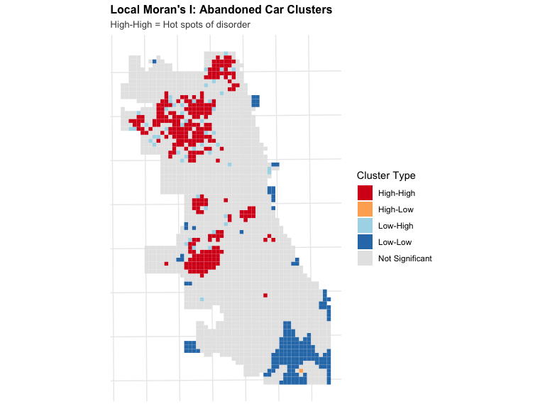
Critical Interpretation of Hotspots

What you’ve identified:

Statistically significant clusters of high abandoned car reports

What this MIGHT mean:

Actual concentrations of abandoned cars
Areas where residents report more (higher civic engagement?)
Areas with more 311 system awareness
Areas with more code enforcement presence
Gentrifying areas with new residents calling on existing conditions

Critical question:

Are these “high abandoned car” areas or “high reporting” areas?

For modeling:

We’re using this as a proxy for “disorder” but recognize it’s a flawed proxy

Part 7B: Count Regression Fundamentals

Why Count Regression? The Problem with OLS

Our outcome: Burglary counts per grid cell (0, 1, 2, 3, …)

Linear regression assumes:

\[Y_i = \beta_0 + \beta_1 X_{1i} + \beta_2 X_{2i} + \varepsilon_i\]

where $\varepsilon_i \sim N(0, \sigma^2)$

Problems for counts:

Can predict negative values (impossible for counts)
Assumes constant variance (counts often have variance ≠ mean)
Assumes continuous outcome (counts are discrete)
Assumes normal errors (count data is skewed)

Distribution of Crime Counts

# Typical pattern for crime data
ggplot(fishnet, aes(x = countBurglaries)) +
  geom_histogram(binwidth = 1, fill = "#440154FF", color = "white") +
  labs(
    title = "Distribution of Burglary Counts",
    subtitle = "Most cells have 0-2 burglaries, few have many",
    x = "Burglaries per Cell",
    y = "Number of Cells"
  ) +
  theme_minimal()

Characteristics:

Right-skewed: Long tail to the right
Many zeros: Most cells have no burglaries
Discrete: Only integer values
Variance > Mean: Overdispersion common

The Poisson Distribution

Appropriate for count data:

\[P(Y = k) = \frac{\lambda^k e^{-\lambda}}{k!}\]

Where:

$Y$ = count outcome (0, 1, 2, …)
$\lambda$ = expected count (mean = variance)
$k$ = observed count

Key property: Mean = Variance = $\lambda$

Examples:

Number of crimes per week
Number of 911 calls per hour
Number of accidents per intersection

Poisson Regression Model

Link $\lambda$ to predictors via log link:

\[\log(\lambda_i) = \beta_0 + \beta_1 X_{1i} + \beta_2 X_{2i} + ... + \beta_p X_{pi}\]

Equivalently:

\[\lambda_i = \exp(\beta_0 + \beta_1 X_{1i} + \beta_2 X_{2i} + ... + \beta_p X_{pi})\]

Why log link?

Ensures $\lambda_i > 0$ (counts can’t be negative)
Linear relationship on log scale
Multiplicative effects on count scale

Interpreting Poisson Coefficients

On log scale:

$\beta_1$ = change in log(expected count) per unit increase in $X_1$

On count scale (exponentiate):

$\exp(\beta_1)$ = multiplicative effect on expected count

Examples:

$\beta$	$\exp(\beta)$	Interpretation
0.14	1.15	15% increase per unit of X
-0.22	0.80	20% decrease per unit of X
0.00	1.00	No effect
0.69	2.00	Doubling per unit of X

Poisson Regression in R

# Fit Poisson model
model_poisson <- glm(
  countBurglaries ~ Abandoned_Cars + Abandoned_Cars.nn + abandoned.isSig.dist,
  data = fishnet,
  family = poisson(link = "log")
)

# View results
summary(model_poisson)

# Exponentiate coefficients for interpretation
exp(coef(model_poisson))

# Example output:
#                        exp(coef)
# (Intercept)            0.234
# Abandoned_Cars         1.151
# Abandoned_Cars.nn      0.998
# abandoned.isSig.dist   0.999

# Interpretation:
# - Each additional abandoned car → 15.1% increase in expected burglaries
# - Each meter from nearest abandoned car → 0.2% decrease in expected burglaries

The Overdispersion Problem

Poisson assumption: Variance = Mean

Reality with crime data: Variance > Mean (often MUCH larger)

Why overdispersion occurs:

Unobserved heterogeneity: Some areas have unmeasured crime attractors
Contagion effects: One crime leads to others (not independent)
Measurement error: Counting issues, data quality
Model misspecification: Missing important variables

Check for overdispersion:

\[\text{Dispersion} = \frac{\text{Residual Deviance}}{\text{Degrees of Freedom}}\]

If ≈ 1: Poisson is fine
If > 1: Overdispersion (common!)
If > 2-3: Serious overdispersion → Use Negative Binomial

Checking Overdispersion in R

# Fit Poisson model
model_pois <- glm(
  countBurglaries ~ Abandoned_Cars + Abandoned_Cars.nn + abandoned.isSig.dist,
  data = fishnet,
  family = poisson
)

# Calculate dispersion parameter
dispersion <- sum(residuals(model_pois, type = "pearson")^2) / 
               model_pois$df.residual

cat("Dispersion parameter:", round(dispersion, 3), "\n")

# Rule of thumb:
# < 1.5: Poisson OK
# 1.5 - 3: Mild overdispersion, NegBin recommended
# > 3: Serious overdispersion, NegBin essential

# Example output:
# Dispersion parameter: 4.523
# Warning: Serious overdispersion detected!

Negative Binomial Regression

Relaxes the variance = mean assumption

Adds dispersion parameter ($\alpha$):

\[\text{Var}(Y_i) = \mu_i + \alpha \mu_i^2\]

Where:

$\mu_i$ = expected count (same as Poisson)
$\alpha$ = dispersion parameter

If $\alpha = 0$: Reduces to Poisson

If $\alpha > 0$: Allows extra variance (overdispersion)

Interpretation: Coefficients interpreted same way as Poisson!

Negative Binomial in R

library(MASS)

# Fit Negative Binomial model
model_nb <- glm.nb(
  countBurglaries ~ Abandoned_Cars + Abandoned_Cars.nn + abandoned.isSig.dist,
  data = fishnet
)

# View results
summary(model_nb)

# Compare to Poisson
AIC(model_pois)  # e.g., 8234.5
AIC(model_nb)    # e.g., 6721.3

# Lower AIC = better fit
# If NegBin AIC much lower → use NegBin

# Extract dispersion parameter (theta)
model_nb$theta  # e.g., 2.47

# Interpretation: Significant overdispersion confirmed

Comparing Poisson vs. Negative Binomial

Aspect	Poisson	Negative Binomial
Variance assumption	Var = Mean	Var = μ + αμ²
Overdispersion	Cannot handle	Accommodates
Standard errors	Underestimated if overdispersed	Correctly estimated
When to use	Count data, no overdispersion	Count data with overdispersion
Crime data	Rarely appropriate	Usually better

For today’s lab: We’ll fit both, compare, and use the better model

Model Diagnostics for Count Models

Unlike OLS, we don’t use residual plots the same way

Key diagnostics:

Dispersion test (already covered)
Deviance residuals: Should be roughly normal
Pearson residuals: Check for outliers
Cook’s distance: Influential observations
Predicted vs. observed: Visual check

# Deviance residuals
plot(model_nb, which = 1)  # Residuals vs. Fitted

# Identify outliers
outliers <- which(abs(residuals(model_nb, type = "deviance")) > 3)

# Influence
influence <- cooks.distance(model_nb)
influential <- which(influence > 4/length(influence))

Part 7C: Spatial Features for Predictive Modeling

Why Add Spatial Features?

Basic model:

\[\log(\lambda_i) = \beta_0 + \beta_1 (\text{Abandoned Cars}_i)\]

Problem: Ignores spatial context

Enhanced model with spatial features:

\[\log(\lambda_i) = \beta_0 + \beta_1 (\text{Abandoned Cars}_i) + \beta_2 (\text{Distance to Nearest}_i) + \beta_3 (\text{Distance to Hotspot}_i)\]

Benefits:

Captures spillover effects
Accounts for spatial dependence
Improves predictions
More realistic model of spatial crime processes

Distance to Nearest Feature

Concept: Proximity matters for risk

Implementation: k-Nearest Neighbors (k=1)

For each grid cell:

Find location of all abandoned cars
Calculate distance to each
Keep minimum distance

In R:

library(FNN)

# Calculate distance to nearest abandoned car
nn_dist <- get.knnx(
  data = st_coordinates(abandoned_cars),      # "To" locations
  query = st_coordinates(st_centroid(fishnet)), # "From" locations
  k = 1                                          # Nearest 1
)

# Extract distances
fishnet$abandoned_car_nn <- nn_dist$nn.dist[, 1]

Distance to Hotspot

Two-step process:

Step 1: Identify hotspots (Local Moran’s I High-High clusters)

Step 2: Calculate distance from each cell to nearest hotspot

# Step 1: Identify hotspots (we did this earlier)
hotspot_cells <- filter(fishnet, hotspot == 1)

# Step 2: Calculate distances
hotspot_dist <- get.knnx(
  data = st_coordinates(st_centroid(hotspot_cells)),
  query = st_coordinates(st_centroid(fishnet)),
  k = 1
)

fishnet$hotspot_nn <- hotspot_dist$nn.dist[, 1]

Why useful? Captures multi-scale spatial dependence:

Local (within cell)
Neighborhood (distance to nearest)
Regional (distance to hotspot cluster)

Visualizing Distance Features

# Create comparison maps
p1 <- ggplot(fishnet) +
  geom_sf(aes(fill = abandoned_car_nn), color = NA) +
  scale_fill_viridis_c(name = "Distance (m)", option = "plasma") +
  labs(title = "Distance to Nearest Abandoned Car") +
  theme_void()

p2 <- ggplot(fishnet) +
  geom_sf(aes(fill = hotspot_nn), color = NA) +
  scale_fill_viridis_c(name = "Distance (m)", option = "magma") +
  labs(title = "Distance to Nearest Hotspot") +
  theme_void()

grid.arrange(p1, p2, ncol = 2)

Look for: Concentric patterns around features/hotspots

Part 7D: The Fishnet Grid Approach

Why Use a Fishnet Grid?

Problem: Crime is points, but we need areas for modeling

Options:

Existing boundaries (census tracts, neighborhoods)
- Pro: Align with administrative data
- Con: Arbitrary, unequal sizes, Modifiable Areal Unit Problem
Fishnet grid (regular cells)
- Pro: Consistent size, no boundary bias
- Con: Arbitrary, may split “natural” areas

We use fishnet because:

Standard approach in predictive policing
Easier spatial operations
Consistent unit of analysis

Creating a Fishnet Grid

library(sf)

# Step 1: Define cell size (in map units - meters for our projection)
cell_size <- 500  # 500m x 500m cells

# Step 2: Create grid over study area
fishnet <- st_make_grid(
  chicago_boundary,
  cellsize = cell_size,
  square = TRUE,
  what = "polygons"
) %>%
  st_sf() %>%
  mutate(uniqueID = row_number())

# Step 3: Clip to study area (remove cells outside boundary)
fishnet <- fishnet[chicago_boundary, ]

# Check results
nrow(fishnet)  # Number of cells
st_area(fishnet[1, ])  # Area of one cell (should be 250,000 m²)

Grid Cell Size: A Critical Choice

Common sizes:

250m × 250m: Fine-grained, many cells, computationally intensive
500m × 500m: Standard, balance detail and computation
1000m × 1000m: Coarse, faster, loses local detail

Smaller cells:

✓ More spatial detail
✓ Better capture local patterns
✗ More zeros (sparse data)
✗ Computational cost

Larger cells:

✓ Fewer zeros
✓ More stable estimates
✗ Lose local variation
✗ May obscure hotspots

Choice affects results! No “correct” answer.

Aggregating Points to Grid

Process:

Spatial join between crimes (points) and fishnet (polygons)
Count crimes per cell
Handle cells with zero crimes

# Count burglaries per cell
burglary_counts <- st_join(burglaries, fishnet) %>%
  st_drop_geometry() %>%
  group_by(uniqueID) %>%
  summarize(countBurglaries = n())

# Join back to fishnet
fishnet <- fishnet %>%
  left_join(burglary_counts, by = "uniqueID") %>%
  mutate(countBurglaries = replace_na(countBurglaries, 0))

# Summary
summary(fishnet$countBurglaries)
#   Min. 1st Qu.  Median    Mean 3rd Qu.    Max. 
#      0       0       1    2.3       3      47

Handling Zeros in Count Data

Crime data typically has MANY zeros

Example distribution: - 40% of cells: 0 burglaries - 30% of cells: 1 burglary - 20% of cells: 2-3 burglaries - 10% of cells: 4+ burglaries

Implications:

Poisson handles zeros naturally (built into distribution)
Zero-inflation: If >60% zeros, consider Zero-Inflated Poisson (ZIP)
For today: Standard Negative Binomial handles our zeros fine

Critical interpretation: Are zeros “true zeros” (no crime) or “missing data” (unreported)?

Part 7E: Spatial Cross-Validation

Why Standard Cross-Validation Fails for Spatial Data

Standard k-fold CV:

Randomly split data into k folds
Train on k-1 folds, test on 1
Repeat k times

Problem with spatial data:

Nearby observations are correlated
Training set includes cells adjacent to test cells
Spatial leakage: Model learns from neighbors of test set
Overly optimistic performance estimates

Solution: Spatial cross-validation

Leave-One-Group-Out Cross-Validation (LOGO-CV)

Principle: Hold out entire spatial groups, not individual cells

Process:

Divide study area into groups (e.g., police districts)
Hold out all cells in District 1
Train model on Districts 2-N
Predict for District 1
Repeat for each district

Why better:

Tests generalization to truly new areas
No spatial leakage between train/test
More realistic deployment scenario
Conservative performance estimates

LOGO-CV Implementation

# Get unique districts
districts <- unique(fishnet$District)

# Initialize results
cv_results <- list()

# Loop through districts
for (dist in districts) {
  # Split data
  train_data <- fishnet %>% filter(District != dist)
  test_data <- fishnet %>% filter(District == dist)
  
  # Fit model on training data
  model_cv <- glm.nb(
    countBurglaries ~ Abandoned_Cars + Abandoned_Cars.nn + abandoned.isSig.dist,
    data = train_data
  )
  
  # Predict on test data
  test_data$prediction <- predict(model_cv, test_data, type = "response")
  
  # Store results
  cv_results[[dist]] <- test_data
}

# Combine all predictions
all_predictions <- bind_rows(cv_results)

Evaluating CV Performance

Common metrics for count models:

Mean Absolute Error (MAE): \[MAE = \frac{1}{n}\sum_i |y_i - \hat{y}_i|\]

Root Mean Squared Error (RMSE): \[RMSE = \sqrt{\frac{1}{n}\sum_i (y_i - \hat{y}_i)^2}\]

Mean Error (Bias): \[ME = \frac{1}{n}\sum_i (y_i - \hat{y}_i)\]

# Calculate metrics by district
cv_metrics <- all_predictions %>%
  group_by(District) %>%
  summarize(
    MAE = mean(abs(countBurglaries - prediction)),
    RMSE = sqrt(mean((countBurglaries - prediction)^2)),
    ME = mean(countBurglaries - prediction)
  )

Interpreting Prediction Errors

What do errors tell us?

MAE = 1.5 burglaries per cell:

On average, we’re off by 1.5 burglaries
Interpretable in original units

RMSE = 2.3 burglaries per cell:

Penalizes large errors more
If RMSE >> MAE, we have some very bad predictions

ME = -0.3 burglaries per cell:

Negative: We tend to under-predict
Positive: We tend to over-predict
Close to zero: Unbiased predictions

Critical question: Are errors evenly distributed across neighborhoods?

Spatial Patterns in Prediction Errors

# Map prediction errors
all_predictions <- all_predictions %>%
  mutate(
    error = countBurglaries - prediction,
    abs_error = abs(error),
    pct_error = (prediction - countBurglaries) / (countBurglaries + 1) * 100
  )

# Visualize
ggplot(all_predictions) +
  geom_sf(aes(fill = error), color = NA) +
  scale_fill_gradient2(
    low = "blue", mid = "white", high = "red",
    midpoint = 0,
    name = "Error"
  ) +
  labs(title = "Prediction Errors",
       subtitle = "Red = Over-prediction, Blue = Under-prediction") +
  theme_void()

Look for: Systematic patterns by neighborhood

Part 7F: Comparison to Baseline (Kernel Density)

Why Compare to Kernel Density Estimation?

KDE is the simplest spatial prediction method:

Place smooth “bump” over each crime location
Sum all bumps to create risk surface
No predictors, no model, just past locations

Benefits of comparison:

Benchmark: Does our complex model beat a simple baseline?
Value added: What do spatial features contribute?
Practical: KDE is computationally simpler
Critical: Maybe spatial patterns alone explain everything?

If our model doesn’t beat KDE, we’re wasting complexity

Kernel Density Estimation Explained

Conceptually:

Imagine placing a “hill” over each crime location:

Peak at the crime location
Height decreases with distance
Controlled by bandwidth parameter

Mathematical:

\[\hat{f}(s) = \frac{1}{n\tau^2}\sum_{i=1}^n K\left(\frac{d(s, s_i)}{\tau}\right)\]

Where:

$s$ = location where we estimate density
$s_i$ = location of crime $i$
$\tau$ = bandwidth (smoothing parameter)
$K$ = kernel function (usually Gaussian)
$d(s, s_i)$ = distance between $s$ and $s_i$

Bandwidth Selection: A Critical Choice

Small bandwidth (e.g., 250m):

Narrow bumps
Preserves local detail
Can be “noisy” (overfit to specific locations)

Large bandwidth (e.g., 2000m):

Wide bumps
Smooth, generalized patterns
May miss important local hotspots

Common choices for urban crime:

500m - 1000m (balance local and regional)

Our approach:

Use 1000m (1 km) bandwidth
Standard in predictive policing literature

Calculating KDE in R

library(spatstat)

# Step 1: Convert to point pattern (ppp) object
burglary_ppp <- as.ppp(
  X = st_coordinates(burglaries),
  W = as.owin(st_bbox(chicago_boundary))
)

# Step 2: Calculate KDE
kde_surface <- density.ppp(
  burglary_ppp,
  sigma = 1000,  # Bandwidth in meters
  edge = TRUE    # Edge correction
)

# Step 3: Extract values to fishnet cells
fishnet$kde_risk <- raster::extract(
  raster(kde_surface),
  st_centroid(fishnet)
)

# Standardize to 0-1 scale for comparison
fishnet$kde_risk <- (fishnet$kde_risk - min(fishnet$kde_risk, na.rm=T)) / 
                     (max(fishnet$kde_risk, na.rm=T) - min(fishnet$kde_risk, na.rm=T))

Creating Risk Categories

Both KDE and our model produce continuous risk scores

For evaluation, convert to categories:

# Create quintiles (5 equal groups)
fishnet$model_risk_category <- cut(
  fishnet$prediction,
  breaks = quantile(fishnet$prediction, probs = seq(0, 1, 0.2)),
  labels = c("1st (Lowest)", "2nd", "3rd", "4th", "5th (Highest)"),
  include.lowest = TRUE
)

fishnet$kde_risk_category <- cut(
  fishnet$kde_risk,
  breaks = quantile(fishnet$kde_risk, probs = seq(0, 1, 0.2)),
  labels = c("1st (Lowest)", "2nd", "3rd", "4th", "5th (Highest)"),
  include.lowest = TRUE
)

Each category contains 20% of cells

Testing on Hold-Out Data (2018 Burglaries)

Critical: Test on data the model has NEVER seen

Process:

Train model on 2017 data
Create risk predictions for all cells
Load 2018 burglaries (new data)
Count how many 2018 burglaries fall in each risk category
Compare model vs. KDE

Question: Which method captures more crimes in high-risk areas?

# Spatial join: 2018 burglaries to fishnet with risk categories
results_2018 <- st_join(fishnet, burglaries_2018) %>%
  group_by(model_risk_category) %>%
  summarize(burglaries_2018 = n()) %>%
  mutate(pct_of_total = 100 * burglaries_2018 / sum(burglaries_2018))

The Hit Rate Evaluation

Goal: Capture maximum crimes with minimum resources

Ideal result:

If we patrol the highest-risk 20% of cells (Category 5):

Model: Captures 55% of 2018 burglaries
KDE: Captures 48% of 2018 burglaries

Interpretation:

Model is better (55% > 48%)
But still imperfect (missing 45% of burglaries)
Spatial features add value over location alone

Random patrol: Would capture ~20% (by chance)

Visualizing Model vs. KDE Performance

# Bar chart comparing methods
comparison_data <- bind_rows(
  model_results %>% mutate(Method = "Negative Binomial Model"),
  kde_results %>% mutate(Method = "Kernel Density")
)

ggplot(comparison_data, aes(x = risk_category, y = pct_of_total, fill = Method)) +
  geom_bar(stat = "identity", position = "dodge") +
  scale_fill_manual(values = c("#440154FF", "#FDE724FF")) +
  labs(
    title = "Percentage of 2018 Burglaries Captured",
    subtitle = "Which method performs better in high-risk areas?",
    x = "Risk Category",
    y = "% of Total 2018 Burglaries"
  ) +
  theme_minimal() +
  theme(legend.position = "bottom")

Critical Interpretation of Performance

Statistical Success:

✓ Model beats KDE
✓ Better than random
✓ Statistically significant difference

But ask:

Which neighborhoods are classified as “highest risk”?
What happens when police patrol those areas?
Who experiences increased surveillance?
Are we predicting crime or policing patterns?
Does “better prediction” = “better public safety”?

A technically superior model can still be ethically problematic

Part 7G: Putting It All Together

The Complete Modeling Workflow

Step 1: Data Preparation

Create fishnet grid
Aggregate crimes to cells
Calculate spatial features (Local Moran’s I, distances)

Step 2: Exploratory Analysis

Visualize crime patterns
Check for spatial autocorrelation
Identify hotspots

Step 3: Model Fitting

Fit Poisson (check overdispersion)
Fit Negative Binomial (if overdispersed)
Interpret coefficients

Workflow (Continued)

Step 4: Validation

Spatial cross-validation (LOGO-CV)
Calculate error metrics
Map prediction errors

Step 5: Comparison

Calculate KDE baseline
Test both on hold-out data (2018)
Compare hit rates by risk category

Step 6: Critical Analysis

Interrogate data sources
Identify potential biases
Assess harms and benefits
Propose alternatives

What If We Predicted Differently?

Instead of:

Where will crimes occur? → Deploy police

Consider:

Where is social services need highest? → Deploy resources
Where is community trust lowest? → Invest in legitimacy
Where is opportunity lowest? → Economic development
Where is housing instability highest? → Stabilize residents

Same technical methods, different normative goal

Predictive Models for Justice, Not Policing

Examples:

Predict eviction risk → Provide legal aid proactively
Predict health crisis → Deploy community health workers
Predict school dropout → Intensive support services
Predict food insecurity → Expand access programs

Key differences:

Predictions lead to help, not punishment
False positives = extra support (relatively low harm)
Builds trust instead of eroding it
Addresses root causes

Key Takeaways

Remember:

All crime data is socially constructed - It reflects policing, not just crime
Historical harms persist in data - Dirty data trains biased systems
Vendors are not accountable - Black boxes prevent oversight
Feedback loops amplify inequality - Predictions become self-fulfilling
Technical accuracy ≠ social justice - A “good” model can be ethically terrible
Alternatives exist - We could predict need instead of threat
Your choices matter - How you build models has real consequences

Critical Perspectives on Predictive Policing

Opening Thought

Today’s Critical Questions

Part 1: The Seductive Promise of Predictive Policing

The Sales Pitch

The Technical Evolution

Part 2: The Dirty Data Problem

What Is “Dirty Data”?

The Many Forms of Dirty Data

Case Study 1: “Juking the Stats” - The Wire and Baltimore

Case Study 2: CompStat and NYPD

The Feedback Loop Diagram

Part 3: Technical Fixes Can’t Solve Social Problems

Vendor Claims About Bias Mitigation

Why “Cleaning” The Data Isn’t Enough

The Impossibility of Neutral Crime Data

Comparison: What Gets Policed vs. What Gets Committed

The “Missing” Data Problem

Part 4: Consequences and Harms

Who Bears the Costs?

Part 5: Can Reform Work?

What Consent Decrees Cover (And Don’t Cover)

The Chicago Consent Decree (2019)

Part 6: A Framework for Critical Evaluation

Questions to Ask About Any Predictive Policing System

1. Data Provenance

2. Variable Selection

Questions (Continued)

3. Validation

4. Deployment

Questions (Continued)

5. Transparency & Accountability

6. Alternatives

The Fundamental Question

Technical Foundations

Modeling Workflow

The Core Logic: “Broken Windows Theory”

Part 7A: Understanding Local Spatial Autocorrelation

Global vs. Local Spatial Autocorrelation

Global Measures

Local Measures

Spatial Weights Matrix: The Foundation

Spatial Weights: Contiguity

Spatial Weights: Row Standardization

Global Moran’s I Formula

Local Moran’s I Formula

The Moran Scatterplot

Statistical Significance Testing

Four Types of Significant Clusters

Local Moran’s I in R: Step by Step

Identifying High-High Clusters (Hotspots)

Hotspot Map

Critical Interpretation of Hotspots

Part 7B: Count Regression Fundamentals

Why Count Regression? The Problem with OLS

Distribution of Crime Counts

The Poisson Distribution

Poisson Regression Model

Interpreting Poisson Coefficients

Poisson Regression in R

The Overdispersion Problem

Checking Overdispersion in R

Negative Binomial Regression

Negative Binomial in R

Comparing Poisson vs. Negative Binomial

Model Diagnostics for Count Models

Part 7C: Spatial Features for Predictive Modeling

Why Add Spatial Features?

Distance to Nearest Feature

Distance to Hotspot

Visualizing Distance Features

Part 7D: The Fishnet Grid Approach

Why Use a Fishnet Grid?

Creating a Fishnet Grid

Grid Cell Size: A Critical Choice

Aggregating Points to Grid

Handling Zeros in Count Data

Part 7E: Spatial Cross-Validation

Why Standard Cross-Validation Fails for Spatial Data

Leave-One-Group-Out Cross-Validation (LOGO-CV)