Logistic Regression for Binary Outcomes

Week 10: Introduction to Logistic Regression

Dr. Elizabeth Delmelle

2025-11-10

Opening: A New Kind of Prediction

A Decision with Real Consequences

Scenario: A state corrections department asks you to help predict:

Will someone released from prison be arrested again within 3 years?

Not asking: How many times? How long until?
Asking: Yes or no? Will it happen or not?

Discussion question (1 minute):

• How is this different from predicting home prices?
• Why might they want this prediction?
• What could go wrong?

Part 1: Introduction to Logistic Regression

Where We’ve Been

Weeks 1-7: Linear regression

• Predicting continuous outcomes: home prices, income, population
• Y = β₀ + β₁X₁ + β₂X₂ + … + ε
• Used RMSE to evaluate predictions

Last week: Poisson regression

• Predicting count outcomes: number of crimes
• Different distribution, but still predicting quantities

Today: A fundamentally different question

• Not “how much?” but “will it happen?”
• Binary outcomes: yes/no, 0/1, success/failure
• This requires a completely different approach

What Makes Binary Outcomes Different?

The problem with linear regression for binary outcomes:

Problems:

• Predictions can be > 1 or < 0 (makes no sense for probability!)
• Assumes constant effect across range (not realistic)
• Violates regression assumptions (errors aren’t normal)

Enter: Logistic Regression

The solution: Transform the problem!

Instead of predicting Y directly, predict the probability that Y = 1

The logistic function constrains predictions between 0 and 1:

\[p(X) = \frac{1}{1+e^{-(\beta_0 + \beta_1X_1 + ... + \beta_kX_k)}}\]

Logistic vs. Linear: Visual Comparison

Key difference: Logistic regression produces valid probabilities!

When Do We Use Logistic Regression?

Perfect for binary classification problems in policy:

Criminal Justice:

• Will someone reoffend? (recidivism)
• Will someone appear for court? (flight risk)

Health:

• Will patient develop disease? (risk assessment)
• Will treatment be successful? (outcome prediction)

Economics:

• Will loan default? (credit risk)
• Will person get hired? (employment prediction)

Urban Planning:

• Will building be demolished? (blight prediction)
• Will household participate in program? (uptake prediction)

The Logit Transformation

Behind the scenes: We work with log-odds, not probabilities directly

Odds: \(\text{Odds} = \frac{p}{1-p}\)

Log-Odds (Logit): \(\text{logit}(p) = \ln\left(\frac{p}{1-p}\right)\)

This creates a linear relationship: \[\ln\left(\frac{p}{1-p}\right) = \beta_0 + \beta_1X_1 + \beta_2X_2 + ...\]

Why this matters:

• Coefficients are log-odds (like linear regression!)
• But we interpret as odds ratios when exponentiated: \(e^{\beta}\)
• OR > 1: predictor increases odds of outcome
• OR < 1: predictor decreases odds of outcome

Part 2: Building Our First Logistic Model

Example: Email Spam Detection

Let’s build a simple spam detector to understand the mechanics.

Goal: Predict whether email is spam (1) or legitimate (0)

Predictors: - Number of exclamation marks - Contains word “free” - Email length

# Create example spam detection data
set.seed(123)
n_emails <- 1000

spam_data <- data.frame(
  exclamation_marks = c(rpois(100, 5), rpois(900, 0.5)),  # Spam has more !
  contains_free = c(rbinom(100, 1, 0.8), rbinom(900, 1, 0.1)),  # Spam mentions "free"
  length = c(rnorm(100, 200, 50), rnorm(900, 500, 100)),  # Spam is shorter
  is_spam = c(rep(1, 100), rep(0, 900))
)

# Look at the data
head(spam_data)

  exclamation_marks contains_free    length is_spam
1                 4             1 150.21006       1
2                 7             1 148.00225       1
3                 4             1 199.10099       1
4                 8             0 193.39124       1
5                 9             0  72.53286       1
6                 2             1 252.02867       1

Fitting the Logistic Model

In R, we use glm() with family = "binomial"

# Fit logistic regression
spam_model <- glm(
  is_spam ~ exclamation_marks + contains_free + length,
  data = spam_data,
  family = "binomial"  # This specifies logistic regression
)

# View results
summary(spam_model)

Call:
glm(formula = is_spam ~ exclamation_marks + contains_free + length, 
    family = "binomial", data = spam_data)

Coefficients:
                   Estimate Std. Error z value Pr(>|z|)
(Intercept)         233.048  15015.736   0.016    0.988
exclamation_marks    55.945  53708.285   0.001    0.999
contains_free        46.055  49298.975   0.001    0.999
length               -1.273     81.369  -0.016    0.988

(Dispersion parameter for binomial family taken to be 1)

    Null deviance: 6.5017e+02  on 999  degrees of freedom
Residual deviance: 7.5863e-07  on 996  degrees of freedom
AIC: 8

Number of Fisher Scoring iterations: 25

Interpreting Coefficients

# Extract coefficients
coefs <- coef(spam_model)
print(coefs)

      (Intercept) exclamation_marks     contains_free            length 
       233.048051         55.944824         46.055006         -1.272668 

# Convert to odds ratios
odds_ratios <- exp(coefs)
print(odds_ratios)

      (Intercept) exclamation_marks     contains_free            length 
    1.627356e+101      1.979376e+24      1.003310e+20      2.800833e-01 

Interpretation:

• exclamation_marks: Each additional ! multiplies odds of spam by 1.9793761^{24}
• contains_free: Having “free” multiplies odds by 1.0033099^{20}
  
• length: Each additional character multiplies odds by 0.2801 (shorter = more likely spam)

Making Predictions

The model outputs probabilities:

# Predict probability for a new email
new_email <- data.frame(
  exclamation_marks = 3,
  contains_free = 1,
  length = 150
)

predicted_prob <- predict(spam_model, newdata = new_email, type = "response")
cat("Predicted probability of spam:", round(predicted_prob, 3))

Predicted probability of spam: 1

But now what?

• If probability = 0.723, is this spam or not?
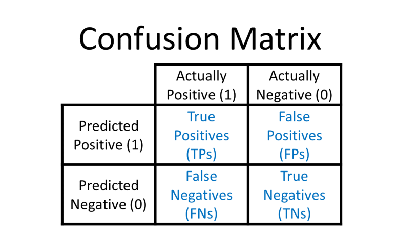
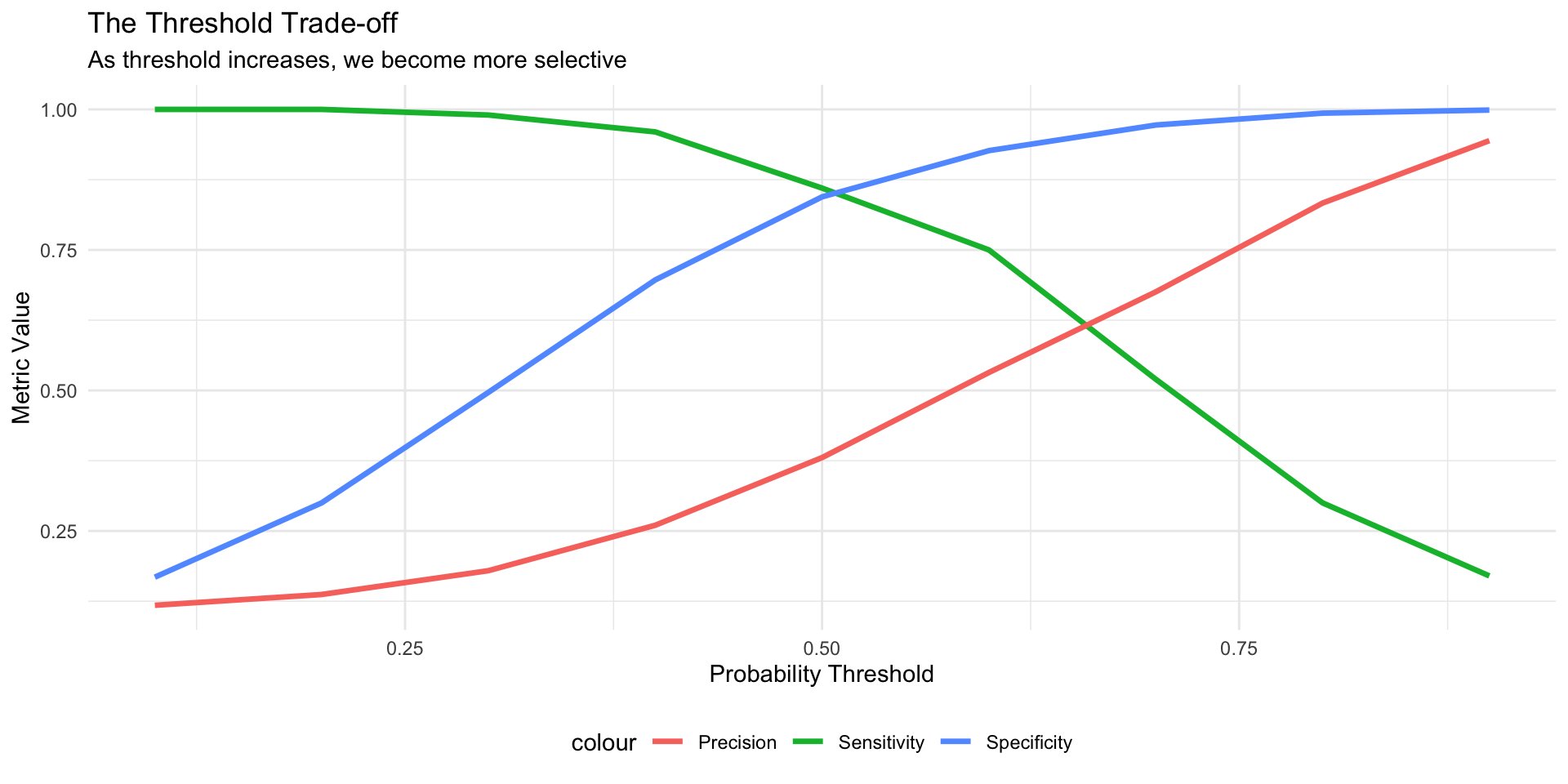
• We need to choose a threshold (cutoff)
• Threshold = 0.5 is common default, but is it the right choice?

The Fundamental Challenge

This is where logistic regression gets interesting (and complicated):

The model gives us probabilities, but we need to make binary decisions.

Question: What probability threshold should we use to classify?

• Threshold = 0.5? (common default)
• Threshold = 0.3? (more aggressive - flag more as spam)
• Threshold = 0.7? (more conservative - only flag obvious spam)

The answer depends on:

• Cost of false positives (marking legitimate email as spam)
• Cost of false negatives (missing actual spam)
• These costs are rarely equal!

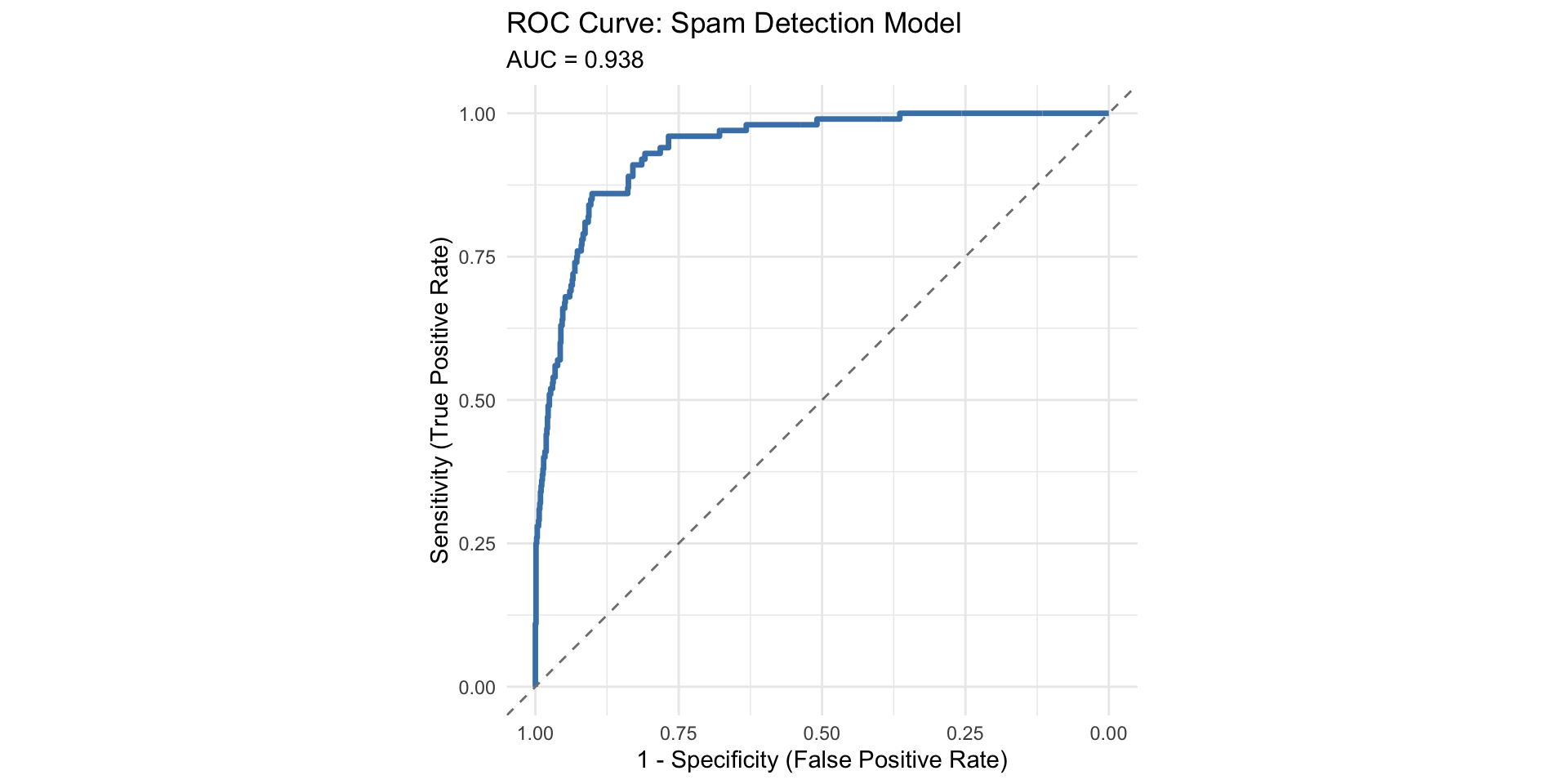
The rest of today: How do we evaluate these predictions and choose thresholds?

Part 3: Evaluating Binary Predictions

From Probabilities to Decisions

We now have a model that predicts probabilities.

But policy decisions require binary choices: spam/not spam, approve/deny, intervene/don’t intervene.

This requires two steps:

1. Choose a threshold to convert probabilities → binary predictions
2. Evaluate how good those predictions are

The confusion matrix helps us with step 2

Part 3a: Confusion Matrices

The Four Outcomes

When we make binary predictions, four things can happen:

Model says “Yes”:

• True Positive (TP): Correct! ✓
• False Positive (FP): Wrong - Type I error

Model says “No”:

• True Negative (TN): Correct! ✓
  
• False Negative (FN): Wrong - Type II error

Confusion Matrix Structure

Remember: The model predicts probabilities. WE choose the threshold that converts probabilities to yes/no predictions.

Quick Example: COVID Testing

Scenario: Testing for COVID-19

COVID Test Outcomes

True_Status	Test_Result	Outcome	Consequence
Positive	Positive	True Positive (TP)	Quarantine (correct)
Positive	Negative	False Negative (FN)	Goes to work, spreads virus
Negative	Positive	False Positive (FP)	Quarantines unnecessarily
Negative	Negative	True Negative (TN)	Goes to work (correct)

Which error is worse?

• False Negative → Virus spreads
• False Positive → Unnecessary quarantine

The answer depends on context! (And changes our threshold choice)

Calculating Performance Metrics

From the confusion matrix, we derive metrics that emphasize different trade-offs:

Sensitivity (Recall, True Positive Rate): \[\text{Sensitivity} = \frac{TP}{TP + FN}\] “Of all actual positives, how many did we catch?”

Specificity (True Negative Rate): \[\text{Specificity} = \frac{TN}{TN + FP}\] “Of all actual negatives, how many did we correctly identify?”

Precision (Positive Predictive Value): \[\text{Precision} = \frac{TP}{TP + FP}\] “Of all our positive predictions, how many were correct?”

Interactive Example: Spam Detection

Let’s say we have an email spam filter:

• 100 actual spam emails
• 900 actual legitimate emails
• Our model makes predictions…

# Create example predictions
set.seed(123)
spam_data <- data.frame(
  actual_spam = c(rep(1, 100), rep(0, 900)),
  predicted_prob = c(rnorm(100, 0.7, 0.2), rnorm(900, 0.3, 0.2))
) %>%
  mutate(predicted_prob = pmax(0.01, pmin(0.99, predicted_prob)))

# With threshold = 0.5
spam_data <- spam_data %>%
  mutate(predicted_spam = ifelse(predicted_prob > 0.5, 1, 0))

# Calculate confusion matrix
conf_mat <- confusionMatrix(
  as.factor(spam_data$predicted_spam),
  as.factor(spam_data$actual_spam),
  positive = "1"
)

Spam Filter Results

          Reference
Prediction   0   1
         0 760  14
         1 140  86

Sensitivity: 0.86 - We caught 86 % of spam

Specificity: 0.844 - We correctly identified 84.4 % of legitimate emails

Precision: 0.381 - Of emails marked spam, 38.1 % actually were spam

Question: What happens if we change the threshold?

Part 4: The Threshold Decision

Why Threshold Choice Matters

Remember: The model gives us probabilities. We decide what probability triggers action.

Threshold = 0.3 (low bar) - More emails marked as spam - Higher sensitivity (catch more spam) - Lower specificity (more false alarms)

Threshold = 0.7 (high bar) - Fewer emails marked as spam - Lower sensitivity (miss some spam) - Higher specificity (fewer false alarms)

There is no “right” answer - it depends on the costs of each type of error

The Great Sensitivity-Specificity Trade-off

# Calculate metrics at different thresholds
thresholds <- seq(0.1, 0.9, by = 0.1)

metrics_by_threshold <- map_df(thresholds, function(thresh) {
  preds <- ifelse(spam_data$predicted_prob > thresh, 1, 0)
  cm <- confusionMatrix(as.factor(preds), as.factor(spam_data$actual_spam), 
                        positive = "1")
  
  data.frame(
    threshold = thresh,
    sensitivity = cm$byClass["Sensitivity"],
    specificity = cm$byClass["Specificity"],
    precision = cm$byClass["Precision"]
  )
})

# Visualize the trade-off
ggplot(metrics_by_threshold, aes(x = threshold)) +
  geom_line(aes(y = sensitivity, color = "Sensitivity"), size = 1.2) +
  geom_line(aes(y = specificity, color = "Specificity"), size = 1.2) +
  geom_line(aes(y = precision, color = "Precision"), size = 1.2) +
  labs(title = "The Threshold Trade-off",
       subtitle = "As threshold increases, we become more selective",
       x = "Probability Threshold", y = "Metric Value") +
  theme_minimal() +
  theme(legend.position = "bottom")

Two Policy Scenarios

Scenario A: Rare, deadly disease screening

• Disease is rare but fatal if untreated
• Treatment is safe with minor side effects
• Goal: Don’t miss any cases (high sensitivity)
• Acceptable: Some false positives (low threshold)

Scenario B: Identifying “high-risk” individuals for intervention

• Limited intervention slots
• False positives waste resources
• False negatives miss opportunities to help
• Goal: Use resources efficiently (high precision)
• Decision depends on: Cost of intervention vs. cost of missed case

Class discussion: Which metrics matter most for each scenario?

Part 5: ROC Curves

The ROC Curve: Visualizing All Thresholds

ROC = Receiver Operating Characteristic

(Originally developed for radar signal detection in WWII)

What it shows:

• Every possible threshold
• Trade-off between True Positive Rate (Sensitivity) and False Positive Rate (1 - Specificity)
• Overall model discrimination ability

How to read it:

• X-axis: False Positive Rate (1 - Specificity)
• Y-axis: True Positive Rate (Sensitivity)
• Diagonal line: Random guessing
• Top-left corner: Perfect prediction

Creating an ROC Curve

# Create ROC curve for our spam example
roc_obj <- roc(spam_data$actual_spam, spam_data$predicted_prob)

# Plot it
ggroc(roc_obj, color = "steelblue", size = 1.2) +
  geom_abline(slope = 1, intercept = 1, linetype = "dashed", color = "gray50") +
  labs(title = "ROC Curve: Spam Detection Model",
       subtitle = paste0("AUC = ", round(auc(roc_obj), 3)),
       x = "1 - Specificity (False Positive Rate)",
       y = "Sensitivity (True Positive Rate)") +
  theme_minimal() +
  coord_fixed()

# Print AUC
auc_value <- auc(roc_obj)
cat("\nArea Under the Curve (AUC):", round(auc_value, 3))

Area Under the Curve (AUC): 0.938

Interpreting AUC

AUC (Area Under the Curve) summarizes overall model performance:

• AUC = 1.0: Perfect classifier
• AUC = 0.9-1.0: Excellent
• AUC = 0.8-0.9: Good
• AUC = 0.7-0.8: Acceptable
• AUC = 0.6-0.7: Poor
• AUC = 0.5: No better than random guessing
• AUC < 0.5: Worse than random (your model is backwards!)

Our spam filter AUC = 0.938

Interpretation: The model has good discrimination ability, but…

• AUC doesn’t tell us which threshold to use
• AUC doesn’t account for class imbalance
• AUC doesn’t show us equity implications

Understanding the ROC Curve Points

Part 6: Equity Considerations

The Core Problem: Disparate Impact

A model can be “accurate” overall but perform very differently across groups

Example metrics from a recidivism model:

Group	Sensitivity	Specificity	False Positive Rate
Overall	0.72	0.68	0.32
Group A	0.78	0.74	0.26
Group B	0.64	0.58	0.42

Group B experiences:

• Lower sensitivity (more people who will reoffend are missed)
• Lower specificity (more people who won’t reoffend are flagged)
• Higher false positive rate (more unjust interventions)

This is algorithmic bias in action

Real-World Case: COMPAS

COMPAS: Commercial algorithm used in criminal justice to predict recidivism

ProPublica investigation (2016) found:

• Similar overall accuracy for Black and White defendants
• BUT: False positive rates differed dramatically
  • Black defendants: 45% false positive rate
  • White defendants: 23% false positive rate
• Black defendants twice as likely to be incorrectly labeled “high risk”

Result:

• Different threshold needed for different groups to achieve equity
• But single-threshold systems are the norm
• Key insight: Overall accuracy masks disparate impact

How to Choose a Threshold

Framework for Threshold Selection

Step 1: Understand the consequences

• What happens with a false positive?
• What happens with a false negative?
• Are costs symmetric or asymmetric?

Step 2: Consider stakeholder perspectives

• Who is affected by each type of error?
• Do all groups experience consequences equally?

Step 3: Choose your metric priority

• Maximize sensitivity? (catch all positives)
• Maximize specificity? (minimize false alarms)
• Balance precision and recall? (F1 score)
• Equalize across groups?

Step 4: Test multiple thresholds

• Evaluate performance across thresholds
• Look at group-wise performance
• Consider sensitivity analysis

Cost-Benefit Analysis Approach

Assign concrete costs to errors:

Example: Disease screening

• True Positive: Treatment cost $1000, prevent $50,000 in complications
• False Positive: Unnecessary treatment $1000
• True Negative: No cost
• False Negative: Miss disease, $50,000 in complications later

Calculate expected cost at each threshold: \[E[\text{Cost}] = C_{FP} \times FP + C_{FN} \times FN\]

Choose threshold that minimizes expected cost

Note: This assumes we can quantify all costs, which is often impossible for justice/equity concerns

Practical Recommendations

1. Report multiple metrics - not just accuracy
2. Show the ROC curve - demonstrates trade-offs
3. Test multiple thresholds - document your choice
4. Evaluate by sub-group - check for disparate impact
5. Document assumptions - explain why you chose your threshold
6. Consider context - what are the real-world consequences?
7. Provide uncertainty - confidence intervals, not just point estimates
8. Enable recourse - can predictions be challenged?

Most importantly: Be transparent about limitations and potential harms