SEPTA Bus Ridership Prediction in Philadelphia
Identifying Transit Deserts to Help Improve Equity-Focused Investments
2025-12-05
A Tale of Two Neighborhoods
- Charlie in West Philly: long waits, rising population
- Center City: frequent service, stable demand
- Planning relies on past ridership… but neighborhoods are changing
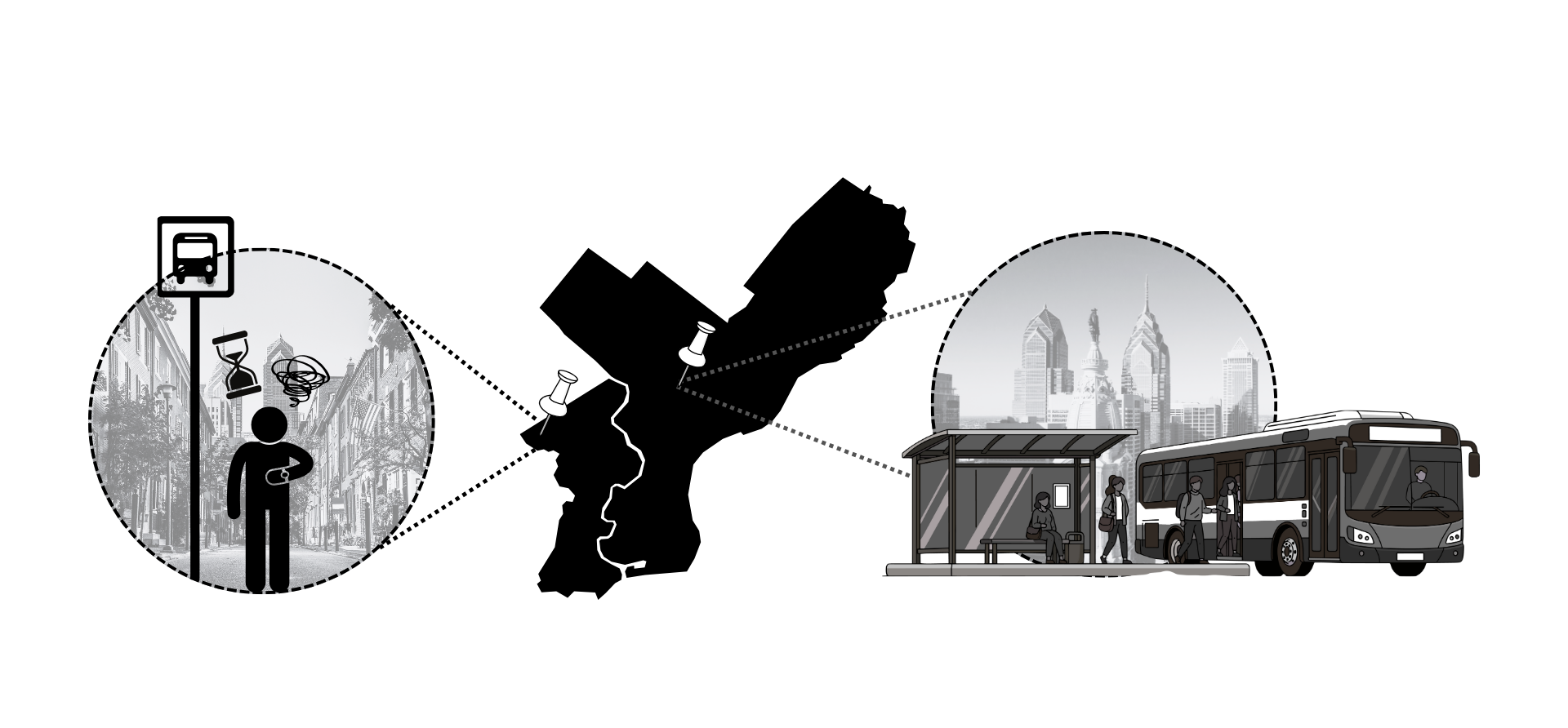
Carlie, who’s waiting for the bus
What Do Ridership Look Like?
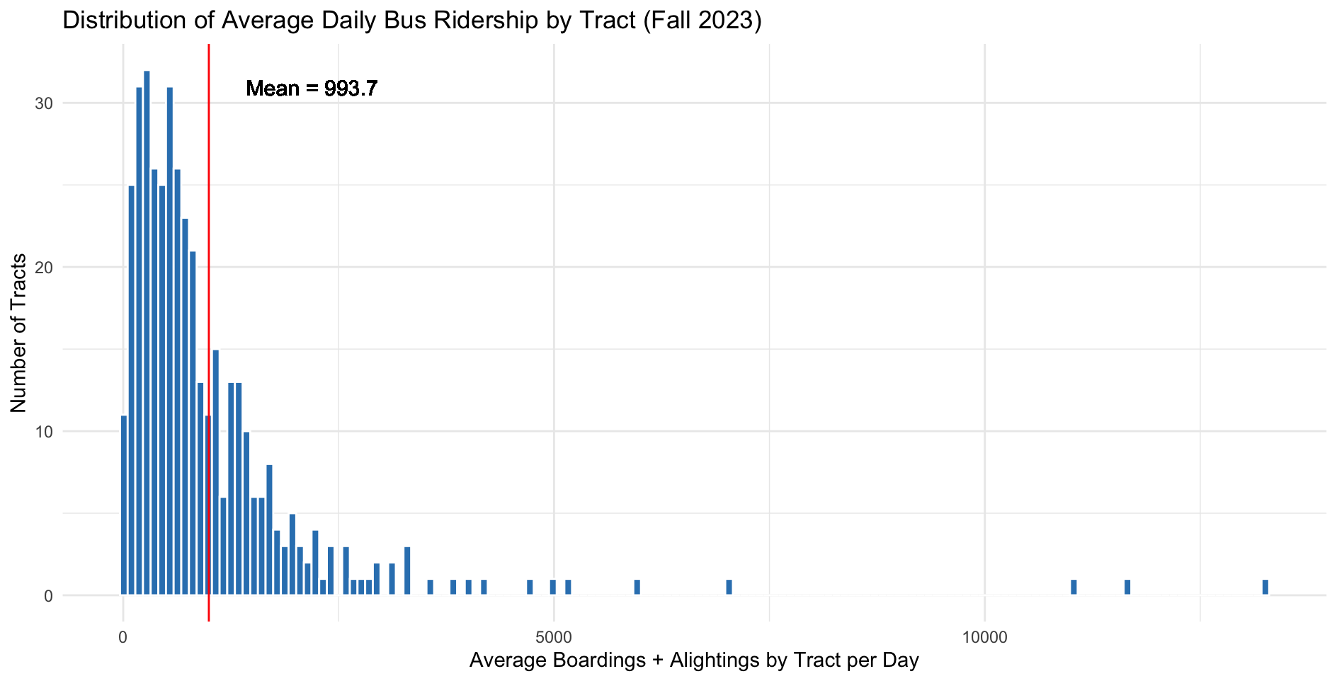
Histogram of Average Bus Ridership by Tract
Key Findings
Most census tracts have relatively low bus activity, while a small number of tracts account for extremely high ridership, creating a heavily skewed distribution.
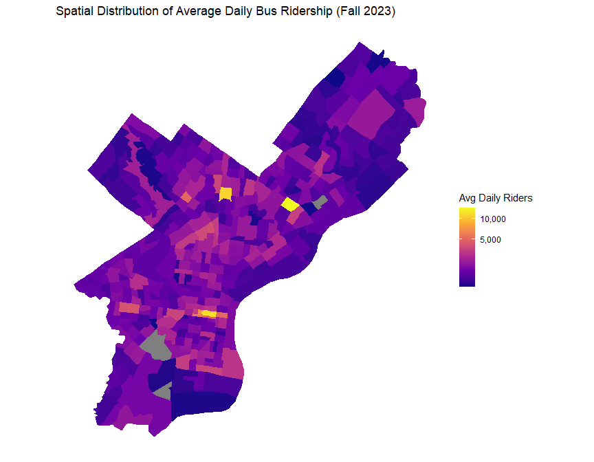
Where Are High Ridership Demands Area?
Key Findings:
- Ridership is highly concentrated in a small number of tracts, shown by the bright yellow hotspots.
- High-ridership areas align with major transit corridors or dense activity centers (e.g., employment hubs, commercial districts).
- Most tracts have relatively low to moderate ridership, reflected by the predominance of darker purple shades.
Ridership & Car Ownership
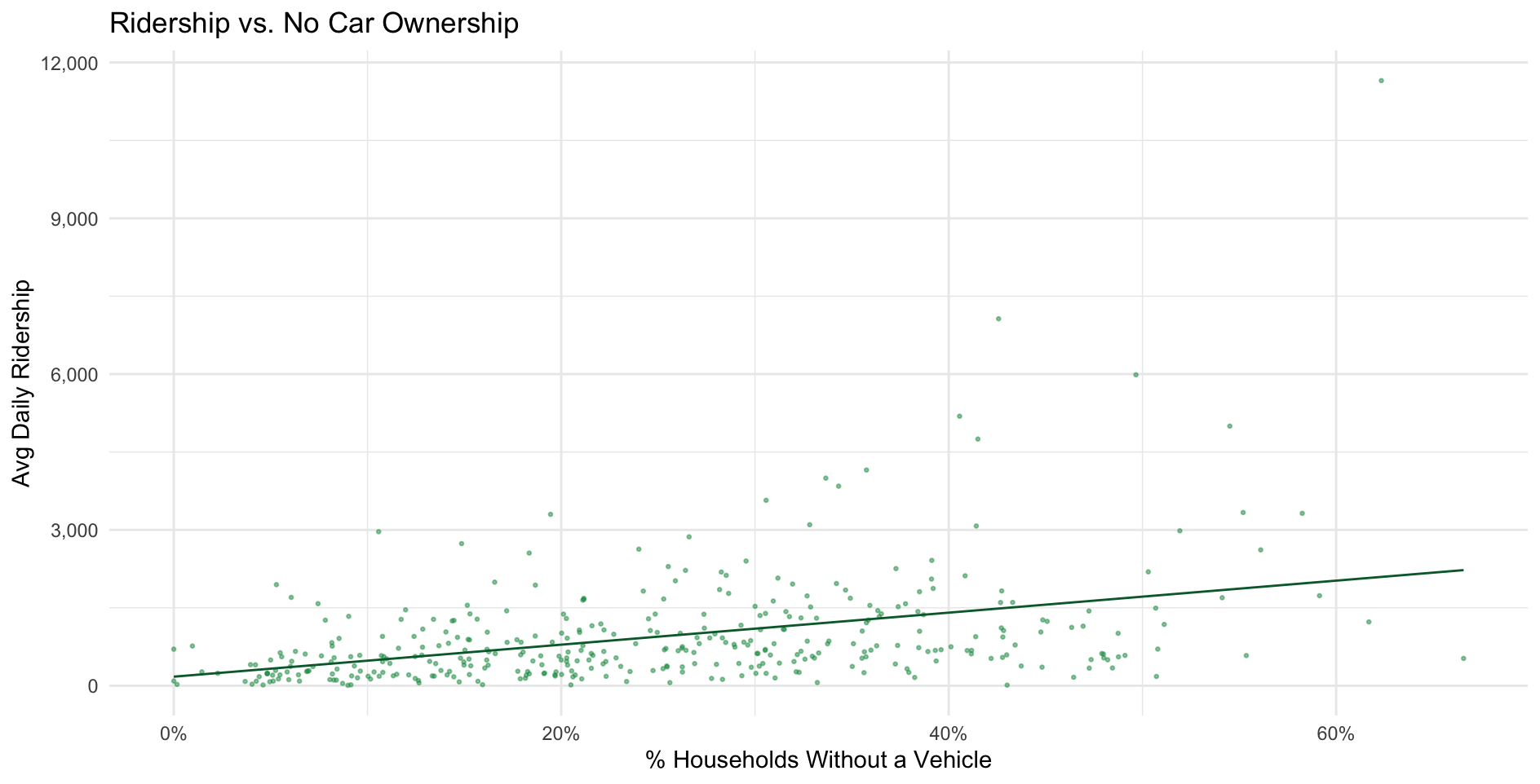
Scatter Map of Bus Ridership vs. Zero Car Ownership by Tract
Key Findings:
- Tracts with higher shares of households without a vehicle show notably higher bus ridership.
- This indicates that household transportation access is a key driver of bus usage.
Ridership & Crime Incidents
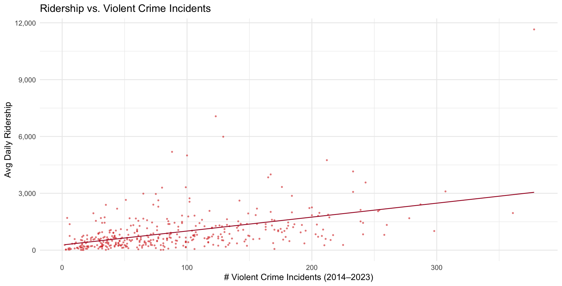
Scatter Map of Bus Ridership vs. Zero Car Ownership by Tract
Key Findings:
- Tracts with more violent incidents tend to have higher bus ridership.
- This likely reflects broader socio-economic conditions rather than crime itself.
Hardest To Predict
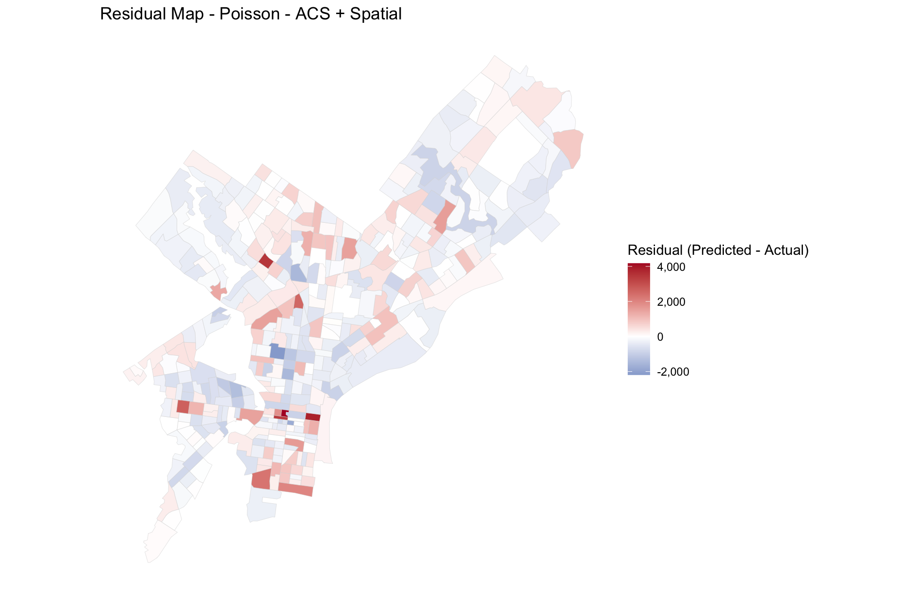
Visualization of Residual by Tract
- Residuals are calculated as actual ridership minus predicted ridership.
- Center city and South Philadelphia have over predicted values, while North and West Philadelphia show under predicted values.
Closing Story: A Better Future Commute
Charlie’s commute:
- Prediction identifies rising demand
- City increases frequency early
- Reliable, shorter commute
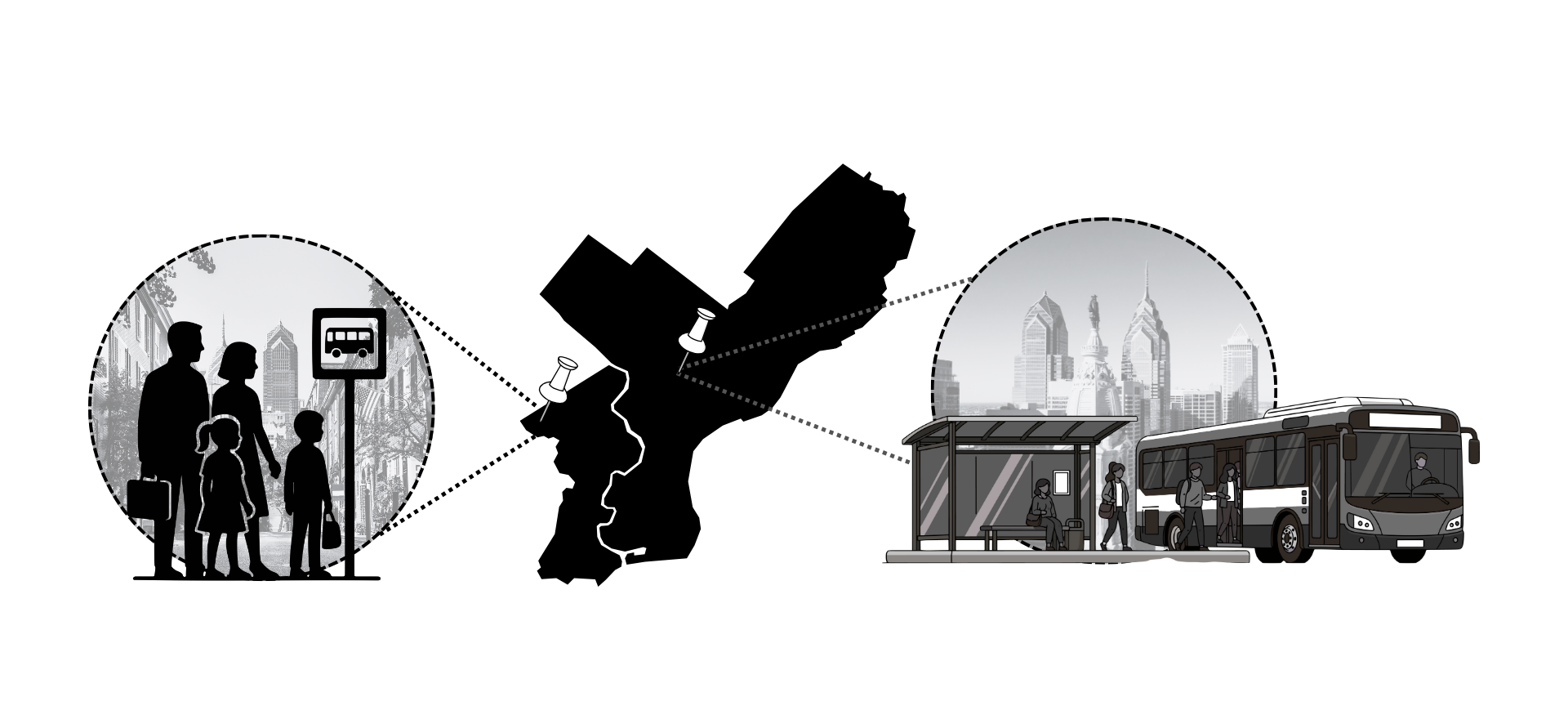
People waiting for the bus