Safe Passage: Optimizing SEPTA Police Deployment

MUSA 5080 Final Project

Xinyuan Cui, Yuqing Yang, Jinyang Xu

2025-12-08

Chapter 1. The Challenge

EYES ON THE STREET OR TARGETS FOR CRIME?

THE PROBLEM: REACTIVE POLICING

SEPTA carries thousands of passengers daily. But for Transit Police, a critical question remains unanswered:

Does high ridership bring safety (“Eyes on the Street”) or does it attract crime (“Potential Targets”)?

🚫 CURRENT ISSUES

  1. Inefficiency: Patrols wasted on safe, high-traffic stops.
  2. Safety Gaps: Missed anomalies where risk is high despite low visibility.
  3. Resource Strain: The “Shotgun approach” fails with limited personnel.

🚨 Our Policy Goal

  • Help SEPTA Transit Police transition from reactive to predictive deployment.

  • We identify “High-Risk Anomalies”—stops where environmental context and timing converge to create danger.

Data Sources: The “Secret Ingredient”

🚌 Operational Data

SEPTA Ridership (Summer 2025) (OpenDataPhilly)

  • Aggregated by Stop

  • Key Feature: Weekday vs. Weekend split

  • Role: Measures “Exposure”

🚨 Outcome Variable

Crime Incidents (OpenDataPhilly)

  • Robbery, Assault, Theft

  • Metric: Total Count (Corrected for days)

🏙️ Environment

(OpenDataPhilly)

  • Alcohol Outlets: Crime Generators
  • Street Lights: Guardianship (CPTED)
  • Vacant Land: Broken Windows
  • Police Stations: Response Distance

👥 Demographics

(ACS Data)

  • Poverty Rate, Unemployment, Income

Chapter 2. The Technique

Why Negative Binomial?

Why Not Linear Regression?

The Statistical Reality

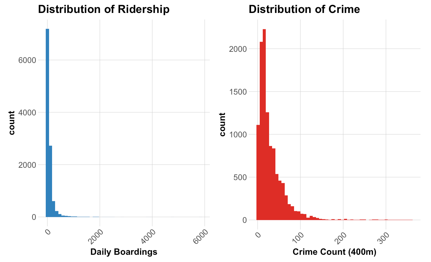
  • The Nature: Crime data is a discrete Count Variable (0, 1, 2…).
  • The Problem: It is heavily Right-Skewed. Most stops have zero crime, creating “Overdispersion” (Variance >> Mean).
  • The Solution: We used Negative Binomial Regression instead of OLS to mathematically account for this distribution.

The Core Hypothesis: Guardian or Target?

Unmasking the Dual Nature of Ridership

We suspect ridership plays competing roles in public safety. A simple regression averages these effects, potentially hiding the truth.

Method: Split the data into Weekdays and Weekends, and use the interaction term to isolate the impact of Ridership.

  • Scenario A (Eyes on the Street): Commuters create natural surveillance.
    • Expectation: Higher ridership \(\rightarrow\) Less Crime.
  • Scenario B (Potential Targets): Leisure crowds create opportunities for theft.
    • Expectation: Higher ridership \(\rightarrow\) More Crime.

The Model Specification:

\[Crime = \beta_0 + \underbrace{\beta_1(Ridership)}_{\text{Guardian Effect}} + \beta_2(Weekend) + \underbrace{\mathbf{\beta_3(Ridership \times Weekend)}}_{\text{Target Effect (The Shift)}}\]

Chapter 3. The EVIDENCE

MODEL PERFORMANCE

WHAT DRIVES CRIME RISK?

🔥 RISK AMPLIFIERS

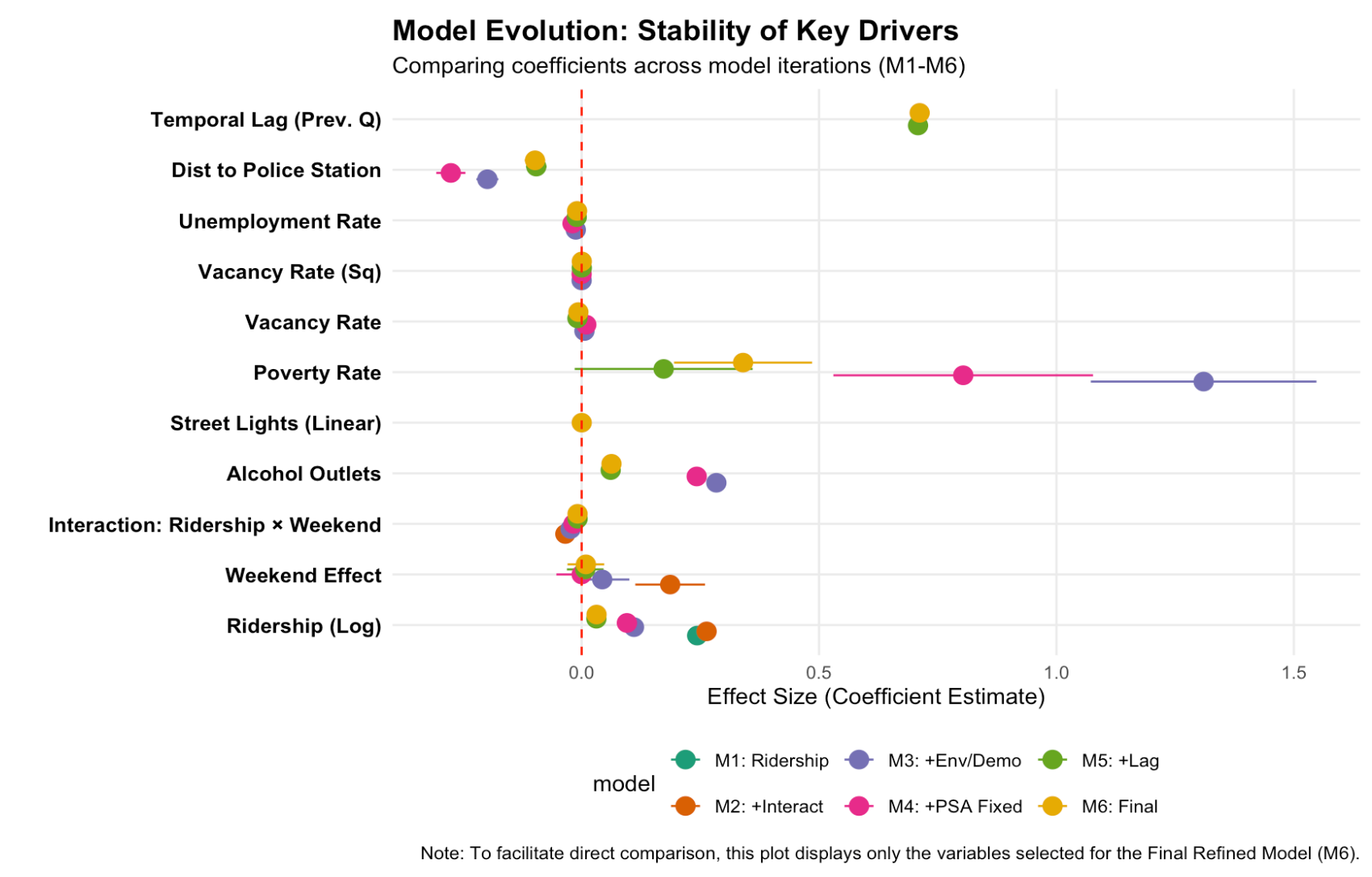
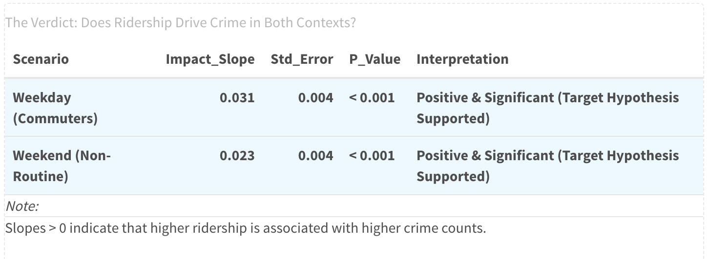
  • Ridership: More people = More targets.
  • Alcohol Outlets: Strongest environmental predictor.
  • Vacancy: “Broken Windows” effect attracts crime.
  • Weekend Shift: The interaction term confirms risk dynamics intensify on weekdays.

🛡️ RISK MITIGATORS

  • Street Lights: Validates CPTED theory—better lighting significantly reduces incidents.

Model Validation (CV Results)

Model Performance Improves with Each Layer

Model MAE (Error Count) RMSE Improvement
1. Ridership Only 17.268 28.877 -
2. + Interaction 17.209 28.868 + 0.3%
3. + Env & Demo 12.777 21.039 + 26%
4. + Fixed 11.409 18.343 + 33.9%
5. + Temporal Lag 7.453 11.629 + 56.8%
6. Refined 7.475 11.662 + 56.7%

Conclusion

Context Matters. Adding environmental variables and temporal lags reduced prediction error by 56.7%.

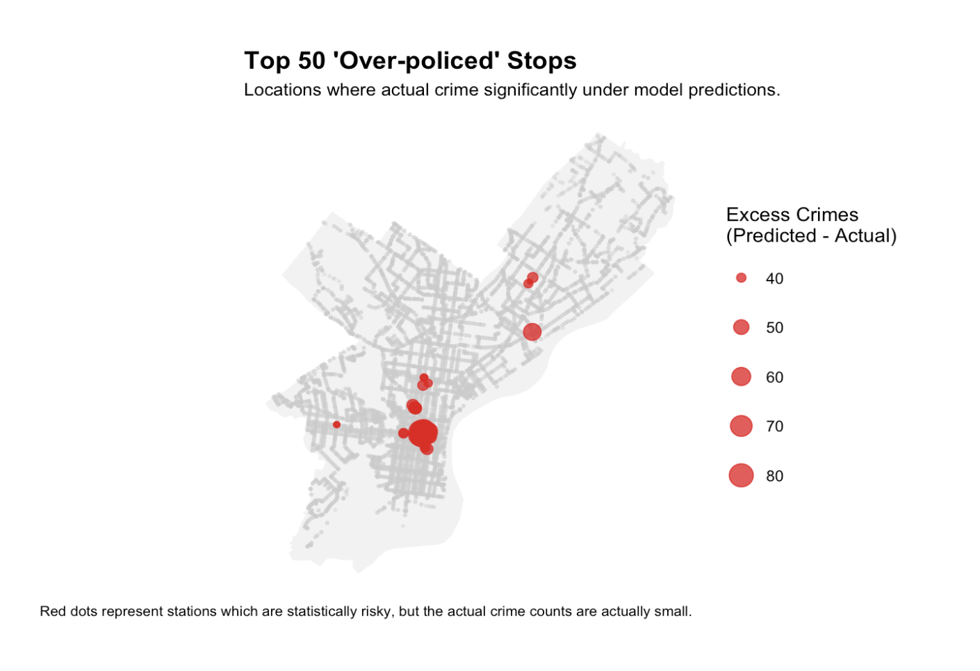
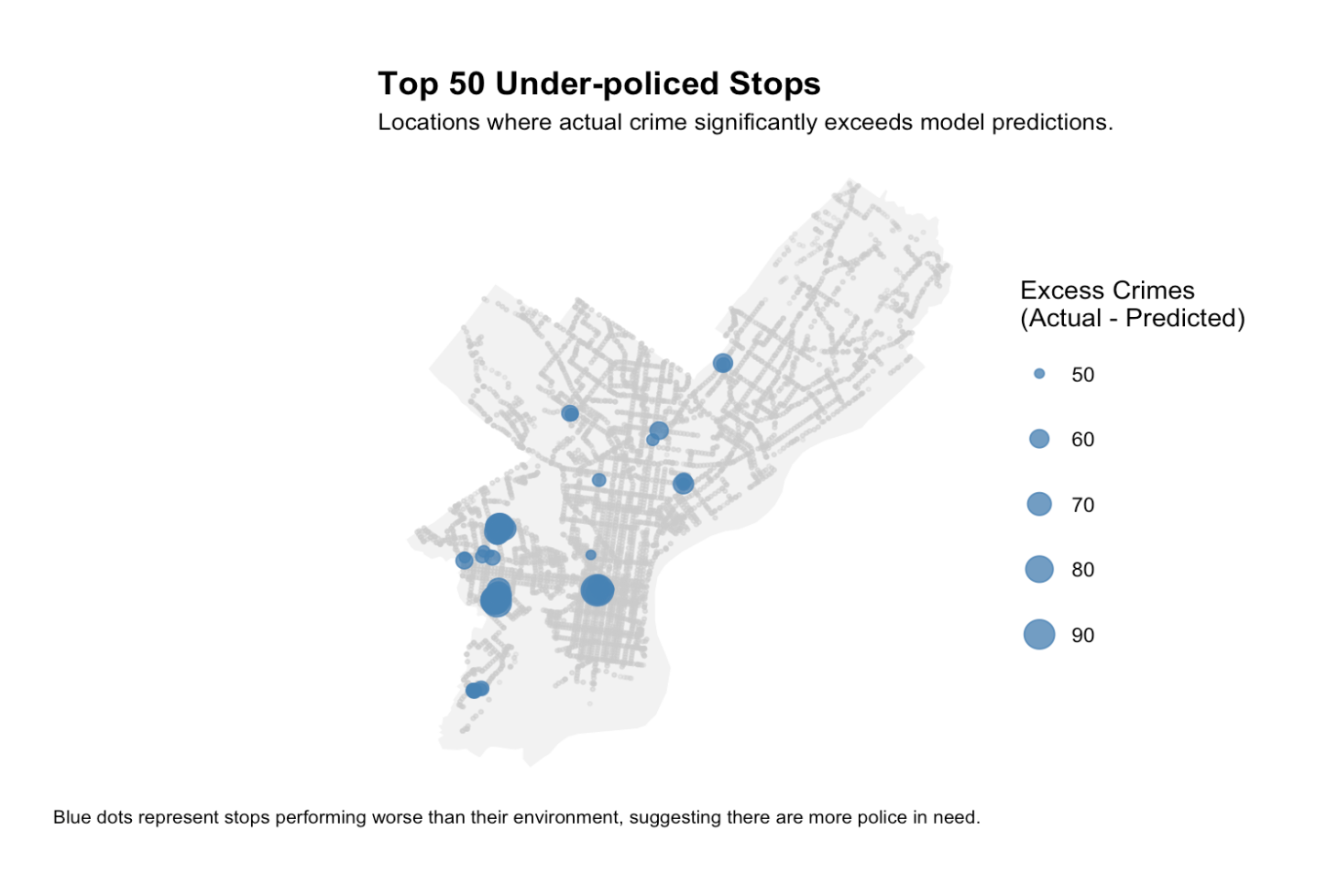
WHERE DOES THE MODEL FAIL? (RESIDUALS)
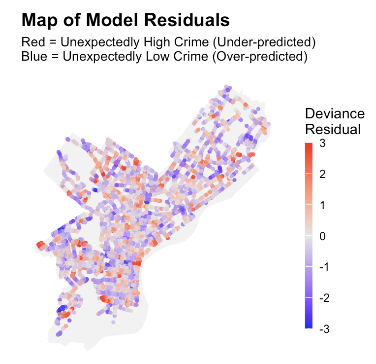
RED ZONES
(UNDER-PREDICTED)

  • Model says “Safe,” Reality is “Dangerous.”
  • Risk: Public safety gaps due to Insufficient Patrols.
  • Action: Needs Human Intelligence.

BLUE ZONES
(OVER-PREDICTED)

  • Model says “Dangerous,” Reality is “Safe.”
  • Risk: Potential for Over-policing in minority neighborhoods.
  • Action: Do not deploy without verification.

Chapter 4. The solution

actionable intelligence

Top 50 Over/Under-Policed Map

🚫 The “Shotgun” Approach Fails

Spreading officers evenly across all high-ridership stops wastes resources on safe stations, while leaving true “High-risk Anomalies” unguarded.
We must distinguish between these scenarios to redeploy effectively.

Implementation

🚀 IMPLEMENTATION

  • Dashboard Integration:
    Embed “Top 50 Risk Map” into HQ command centers. Weekly refresh.
  • Friday Rostering Guide:
    Commanders use the model to shift weekend resources from Commuter Lines to Nightlife Districts.
  • Low Cost Feasibility:
    Uses 100% existing data (SEPTA, Crime, Census). No new sensors required.

🛡️ SAFEGUARDS

  • 1. Graded Response:
    Don’t just send SWAT. Deploy Safety Ambassadors or fix street lights (CPTED) in high-risk zones.
  • 2. Human-in-the-Loop:
    The model is a guide, not a commander. District Captains must validate Red Zones with field intel.
  • 3. Bias Auditing:
    Quarterly checks on Blue Zones to prevent stereotyping low-income areas.

Chapter 5. Critical Analysis

Equity & Bias

LIMITATIONS & EQUITY

⚠️ MODEL LIMITATIONS

  • Unobserved Variables:
    The model cannot capture real-time shocks like temporary gang activity or large events (e.g., concerts).
  • Spatial Lag:
    Crime is fluid. Our 400m buffer is static, potentially missing cross-boundary crime displacement or spillover effects.

⚖️ ALGORITHMIC BIAS

  • The Risk (Over-Policing):
    Reliance on Poverty Rate or Vacancy creates a feedback loop, targeting low-income neighborhoods even when no crime occurs.
  • The Evidence (Blue Zones):
    Our Residual Analysis confirmed this: The model Over-Predicted risk in specific low-income areas, flagging them as dangerous when they were actually safe.

Thank You

Questions?

Team:

Xinyuan Cui | Yuqing Yang | Jinyang Xu