In this analysis, we attempt to measure what factors we can use to predict the sale prices of residential properties in Philadelphia. In order to prepare the dataset for modeling residential property sales, we applied a series of targeted cleaning and structural, socioeconomic, and spatial variable selection.
We filtered our property sales data to only show sales for the past two years to ensure up-to-date insights. We restricted the dataset to "SINGLE FAMILY" and "MULTI FAMILY" homes, excluding apartments and non-residential sales to ensure comparability, relevancy, and accuracy in our prediction models. Various apartments contained within the same building were found to be listed with a comprehensive sales price of the entire building which posed the threat of distorting our analysis. Observation values that were regarded as data entry errors or outliers were also removed. Properties with zero bathrooms, bedrooms, or livable area were removed as well as properties with a sales price below $10,000 and above $1,000,000.
We retained select structural attributes from our original dataset that we considered theoretically relevant to predicting sale price: number of bedrooms, number of bathrooms, total livable area, year the home was built, exterior condition, availability of garage spaces, and finally, the dependent variable, sale price.
Code for Property Sales Data Cleaning and Variable Selection
Code
#load necessary librarieslibrary(modelsummary)library(stargazer)library(sf)library(tigris)library(tidycensus)library(dplyr)library(stringr)library(ggplot2)library(tidyr)library(caret)library(knitr)library(scales)#load census key for later usecensus_api_key("42bf8a20a3df1def380f330cf7edad0dd5842ce6")#save data in url url <-"https://phl.carto.com/api/v2/sql?filename=opa_properties_public&format=geojson&skipfields=cartodb_id&q=SELECT+*+FROM+opa_properties_public"#suppress warnings for clarity and read data as spatial objectsuppressWarnings({ property_data <-st_read(url)})#clean dataparcel_data <- property_data%>%select(location, #load columns that could potentially be used as predictors category_code_description, #maybe garage_spaces and central air too? number_of_bedrooms, number_of_bathrooms, total_livable_area, year_built, exterior_condition, garage_spaces, sale_price, sale_date)%>%filter(category_code_description %in%c("SINGLE FAMILY","MULTI FAMILY"))%>%#no apartments, sales price of buildingdrop_na(number_of_bedrooms, #remove anomalies like houses with no rooms number_of_bathrooms, total_livable_area, sale_price, year_built) %>%filter(number_of_bedrooms>0, number_of_bathrooms>0, total_livable_area>0, sale_price>=10000, sale_price <=1000000)%>%#remove very low/high pricesmutate(sale_year =str_remove(sale_date, "-.*"))%>%filter(sale_year %in%c("2023","2024"))%>%#limit to only 2023 and 2024mutate(year_built =as.numeric(year_built))%>%mutate(Age =2025- year_built)%>%filter(Age <2000)%>%#create a age columnfilter(exterior_condition !=0) %>%#create exterior condition binary mutate(exterior_good =case_when( exterior_condition >=1& exterior_condition <=5~1, exterior_condition >=6& exterior_condition <=9~0,TRUE~NA_real_ ) )
Table 1. Property Dataset Dimensions Before and After Cleaning and Selecting Varaiables
Dataset
Rows
Columns
Raw Property Data
583824
79
Cleaned Parcel Data
25268
14
We derived our socioeconomic predictors from tract-level census data provided by the 2022 American Community Survey: median income, number with at least a bachelor’s degree, total number of those with at least a bachelor’s degree, number of those living in poverty, and total of those living in poverty. Census tracts with missing median income or zero reported as the median income were removed as it often indicated missing or zero values for other key predictors. We also mutated our census dataset to include two more columns, the percentage of people with bachelors and percentage of people in poverty, in order to standardize the observations across varying tract population sizes. Spatial data of the census tracts was also loaded in order to join our census variables to our parcel-level property data.
Code for Census Data Cleaning and Variable Selection
Code
#load data about poverty(counts and total), bachelors(counts and total), and income census_data <-get_acs(geography ="tract",state ="PA",county ="Philadelphia",variables =c(median_income ="B19013_001",num_with_bach ="B15003_022",bachelors_total ="B15003_001",num_in_poverty ="B17001_002",poverty_total ="B17001_001" ),year =2022,output ="wide")#create percentage columns for bachelors and poverty philly_census <- census_data%>%mutate(percentage_bach = num_with_bachE / bachelors_totalE,percentage_pov = num_in_povertyE / poverty_totalE )#remove data errors or incomplete fields philly_census <- philly_census%>%drop_na(median_incomeE)%>%filter(median_incomeE>0)#spatial census data philadelphia_tracts <-tracts(state ="PA",county ="Philadelphia",cb =TRUE,year =2022)#join census data and tract geometry to PARCEL dataparcel_data <- parcel_data %>%st_transform(st_crs(philadelphia_tracts))%>%st_join(philadelphia_tracts, join = st_within)%>%left_join(philly_census, by ="GEOID")
Table 2. Census Dataset Dimensions Before and After Cleaning and Selecting Varaiables
Dataset
Rows
Columns
Census Data
408
12
Cleaned Census Data
383
14
To further contextualize house prices, we loaded spatial datasets including the locations of colleges and universities, 2024 crime incidents, and Philadelphia neighborhood boundaries. These datasets were loaded with the intention of engineering spatial features such as proximity measurements and neighborhood stratification in order to account for spatial patterns and potential interactive spatial effects within our predictive model. Only the 2024 crime incidents needed to be cleaned due to the missing geometries that would prevent spatial analysis.
Code for Spatial Data Cleaning and Variable Selection
Code
#load university datauniversity_data <-st_read("./data/Universities_Colleges.geojson")#load 2024 crime incident dataorg_crime_data <-st_read("./data/incidents_part1_part2.shp")#removed crime incidents with no geometry crime_data <- org_crime_data %>%filter(!st_is_empty(geometry))#load neighborhood data neighborhoods <-st_read("./data/philadelphia-neighborhoods.shp")
Table 3. Spatial Datasets Dimensions Before and After Cleaning
Dataset
Rows
Columns
Crime Data
160388
14
Cleaned Crime Data
153644
14
Phase 2: Exploratory Data Analysis
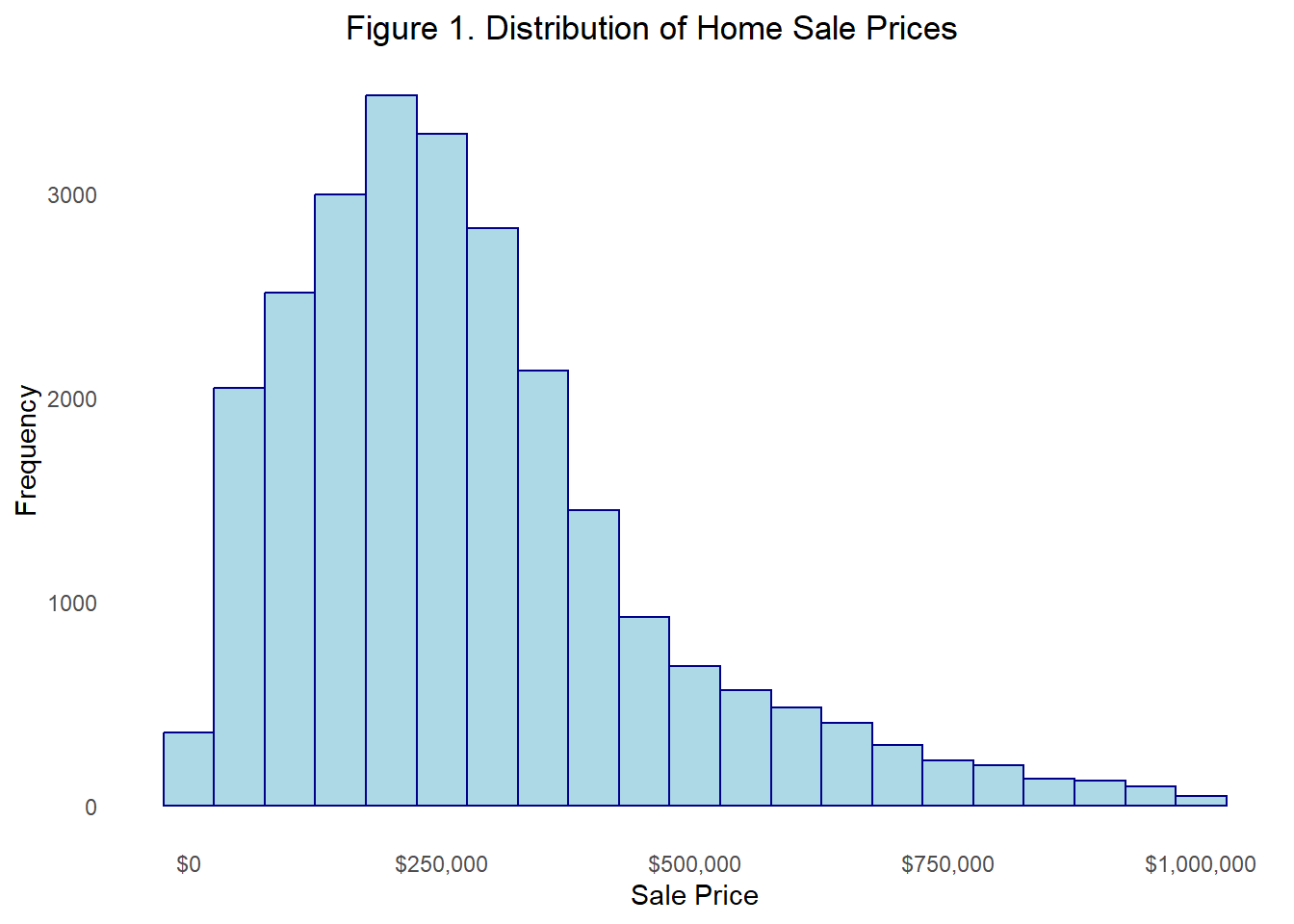
We created a histogram to visualize the distribution of home sale prices in Philadelphia. The resulting graph revealed a positively skewed distribution, indicating that most properties were sold at lower price points, primarily between $150,000 and $350,000, while a small number of high-value homes sold for up to $1,000,000. As it pertains to our predictive model, this skewness suggests that a log-transformation of sale prices may be necessary to normalize the distribution of values and potentially improve model performance. It also indicates the need for diagnostic checks to determine the impact of outliers in order to ensure that the few high-priced homes do not distort our model estimates.
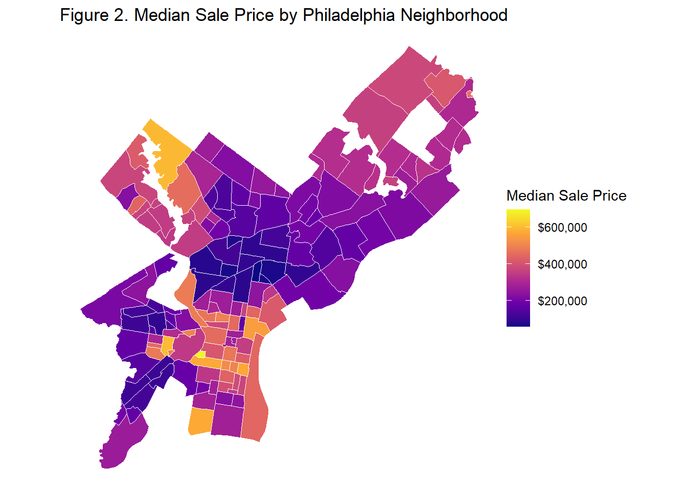
We also explored the geographic distribution of sales prices across the neighborhoods in Philadelphia. We calculated the median sales price by each Philadelphia neighborhood. The map in Figure 2 shows distinct spatial patterns with higher prices above $400,000, represented by lighter colors, being concentrated in neighborhoods such as Center City, University City, and parts of Northwest Philadelphia.
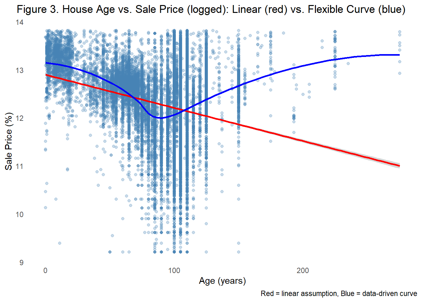
One interesting relationship we found when exploring the structural predictors of sales price was the non-linear association between home age and sale price. Because we have already determined that sale prices are not normally distributed, we plotted our predictors by the log-transformed sale price to limit distortion when attempting to assess the relationship between predictors and sales price. Even with this transformation, Figure 3 shows that sale prices tend to decline for middle-aged homes but rebound for older, more historic properties. The figure includes both a linear and quadratic line to further emphasize that a linear relationship is not sufficient in capturing the impact of age on house prices.
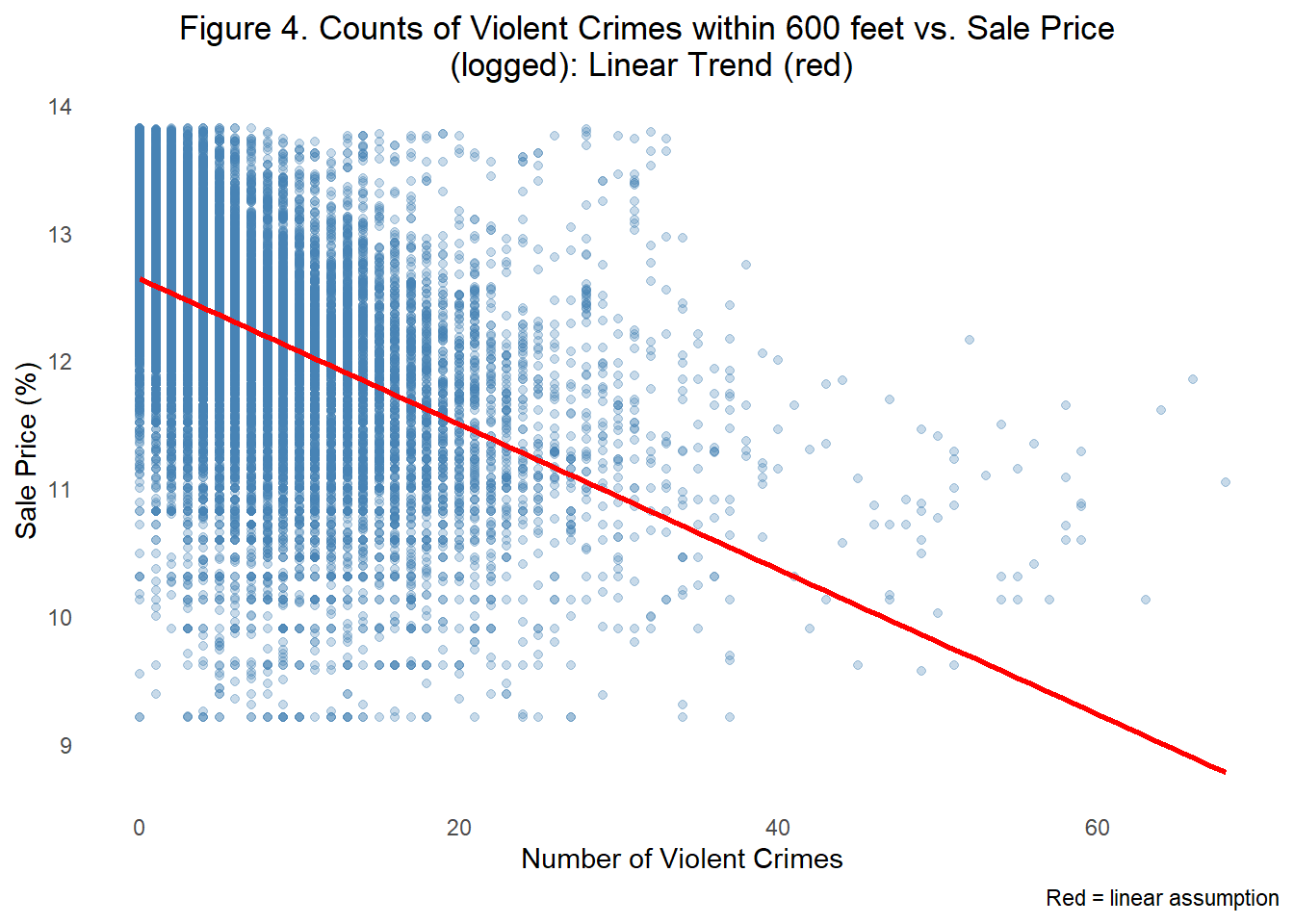
One spatial factor that we found theoretically relevant to predicting sales price was proximity to violent crimes. We hypothesized that a home’s proximity to violent crimes such as homicides, aggravated assaults with and without firearms, and armed robberies may lead to a depreciation in house value. To measure this, loaded the location of crime incidents 2024 and calculated the density of crime within 600 feet of each home. In Figure 4 we explored this relationship between violent crimes and found a general negative trend between proximity to crime and sale price.
We also created a violin plot to illustrates the distribution and density of sale prices across within the top ten neighborhoods with the highest median sale prices. The violin plot in Figure 5 reveals heterogeneity in sale prices within the wealthiest neighborhoods, indicating juxtaposition of high and low sales prices within close proximity of one another. While some neighborhoods are more concentrated at similar sales prices, neighborhoods like Bella Vista and Northern Liberties had long tails extending towards the lowest sale prices.
Phase 3: Feature Engineering
In order to account for the spatial patterns highlight during the exploratory phase, we created a number of spatial features to incorporate into our predictive model.
Code for Feature Engineering: K-Nearest Neighbor for Colleges
Code
#knn to university university_proj <-st_transform(university_data, 3365) #projection changed in order to calculate distance dist_matrix <-st_distance(parcel_proj, university_proj)get_knn_distance <-function(dist_matrix, k) {apply(dist_matrix, 1, function(distances) {mean(as.numeric(sort(distances)[1:k])) })}parcel_data$college_nn1 <-get_knn_distance(dist_matrix, k =1)parcel_data$college_nn3 <-get_knn_distance(dist_matrix, k =3)parcel_data$college_nn5 <-get_knn_distance(dist_matrix, k =5)#determine which nearest neighbor is correlated the most with sales price parcel_data %>%st_drop_geometry() %>%select(sale_price, college_nn1, college_nn3, college_nn5) %>%cor(use ="complete.obs") %>%as.data.frame() %>%select(sale_price)
Code for Feature Engineering: Neighborhood Interaction Effects
Code
# wealthy neighborhood interaction effectsparcel_proj <-st_transform(parcel_data, 3365)neighborhood_proj <-st_transform(neighborhoods, 3365)#median sales price wealthy_neighborhoods <- parcel_with_neighborhood%>%filter(median_price >=275500)%>%pull(NAME)#finding the parcels that fall within neighborhood boundaries parcel_data <- parcel_proj %>%st_join(neighborhood_proj, join = st_within) %>%mutate(wealthy_neighborhood =ifelse(NAME %in% wealthy_neighborhoods, "Wealthy", "Not Wealthy"), #creating a flag to delineate them into two categories wealthy_neighborhood =as.factor(wealthy_neighborhood) )
Table 4. Summary of Engineered Features
Feature_Name
Feature_Type
Description
Justification
violent_crime_600ft
Buffer-based (spatial)
Count of violent crimes within 600 ft of parcel
Captures neighborhood safety and crime exposure
college_nn1
kNN (spatial distance)
Average distance to nearest college/university (k=1)
Measures proximity to educational amenities
college_nn3
kNN (spatial distance)
Average distance to 3 nearest colleges/universities
Captures local educational accessibility
college_nn5
kNN (spatial distance)
Average distance to 5 nearest colleges/universities
Captures broader proximity to higher education hubs
median_incomeE
Census (socioeconomic)
Median household income of census tract
Represents economic conditions of local area
percentage_bach
Census (education)
Percent of tract population with bachelor’s degree
Education level could be connected to property values
percentage_pov
Census (poverty)
Percent of tract population below poverty line
Reflects socioeconomic disadvantage
wealthy_neighborhood
Interaction term (categorical)
Indicates parcels located in wealthy neighborhoods
Identifies context of neighborhood wealth levels
log_sale_price
Transformation (continuous)
Natural log of sale price
Stabilizes variance for regression modeling
log_livable_area
Transformation (continuous)
Natural log of total livable area (sq ft)
Normalizes skewed size variable for modeling
Age
Structural (numeric)
Years since building construction
Accounts for devaluation of property value with time
exterior_good
Condition (binary)
1 = good/average exterior, 0 = poor
Changed categorical condition to numeric to understand exterior desirability
The features included were engineered to capture social, economic, and environmental factors influencing housing prices. Buffer-based and nearest-neighbor measures quantify local accessibility and safety. Census data enrich parcels with socio-economic context. Interaction terms account for neighborhood-level wealth effects which helps contextualize external features of a home, for instance homes in a wealthy neighborhood are more likely to have a higher property value than those not in a wealthy neighborhood. Applying a binary indicator improves model interpretability and performance.
Phase 4: Model Building
When building our model’s be progressively built out models to expand upon the last with out first model being the baseline of all our models and using only structural variables, the second model adding socioeconomic census variables, our third model introducing our spatial features, and our fourth model added spatial interactions and fixed effects.
Code for Model Building
Code
#create log livable area for modelingparcel_data <- parcel_data%>%mutate(log_livable_area =log(total_livable_area))#structural features only model1 <-lm(log_sale_price ~ number_of_bathrooms + number_of_bedrooms + log_livable_area + garage_spaces + Age +I(Age^2) + exterior_good, data = parcel_data)#structural + census model2 <-lm(log_sale_price ~ number_of_bathrooms + number_of_bedrooms + log_livable_area + garage_spaces + Age +I(Age^2) + exterior_good + median_incomeE + percentage_bach + percentage_pov, data = parcel_data)#structural + census + spatial model3 <-lm(log_sale_price ~ number_of_bathrooms+ garage_spaces + Age +I(Age^2) + exterior_good + log_livable_area + median_incomeE +percentage_bach + percentage_pov + college_nn1 + violent_crime_600ft, data = parcel_data)#structural + census + spatial + interactions model4 <-lm(log_sale_price ~ number_of_bathrooms+ garage_spaces + Age +I(Age^2) + exterior_good + log_livable_area * wealthy_neighborhood + median_incomeE +percentage_bach + percentage_pov + college_nn1 + violent_crime_600ft, data = parcel_data)
Our summary table of coefficients for predictors by model indicate statistical numerically as well as with stars to account for low values omitted through the rounding of coefficients.
Full Model Summary of Models
Model 1
Model 2
Model 3
Model 4
(Intercept)
5.512***
7.275***
7.615***
7.175***
[5.254, 5.771]
[7.060, 7.491]
[7.429, 7.802]
[6.933, 7.418]
number_of_bathrooms
0.283***
0.215***
0.213***
0.209***
[0.269, 0.296]
[0.204, 0.226]
[0.202, 0.224]
[0.199, 0.220]
number_of_bedrooms
-0.192***
-0.013*
[-0.204, -0.180]
[-0.023, -0.003]
log_livable_area
0.874***
0.497***
0.461***
0.515***
[0.838, 0.910]
[0.467, 0.528]
[0.437, 0.484]
[0.483, 0.548]
garage_spaces
0.104***
0.098***
0.050***
0.051***
[0.089, 0.119]
[0.085, 0.110]
[0.037, 0.062]
[0.039, 0.064]
Age
-0.012***
-0.004***
-0.004***
-0.003***
[-0.013, -0.011]
[-0.004, -0.003]
[-0.005, -0.003]
[-0.004, -0.003]
I(Age^2)
0.000***
0.000***
0.000***
0.000***
[0.000, 0.000]
[0.000, 0.000]
[0.000, 0.000]
[0.000, 0.000]
exterior_good
1.180***
0.941***
0.881***
0.877***
[1.094, 1.265]
[0.871, 1.011]
[0.813, 0.950]
[0.809, 0.944]
median_incomeE
0.000***
0.000***
0.000***
[0.000, 0.000]
[0.000, 0.000]
[0.000, 0.000]
percentage_bach
1.564***
1.464***
1.051***
[1.474, 1.655]
[1.373, 1.555]
[0.956, 1.147]
percentage_pov
-0.862***
-0.476***
-0.375***
[-0.933, -0.790]
[-0.549, -0.403]
[-0.447, -0.302]
college_nn1
0.000***
0.000***
[0.000, 0.000]
[0.000, 0.000]
violent_crime_600ft
-0.020***
-0.018***
[-0.021, -0.019]
[-0.019, -0.017]
wealthy_neighborhoodWealthy
1.093***
[0.815, 1.372]
log_livable_area × wealthy_neighborhoodWealthy
-0.118***
[-0.157, -0.079]
Num.Obs.
24556
24453
24453
24453
R2
0.351
0.569
0.589
0.600
R2 Adj.
0.350
0.569
0.589
0.600
F
1892.735
3226.742
3189.486
2821.134
RMSE
0.61
0.50
0.48
0.48
p < 0.1, * p < 0.05, ** p < 0.01, *** p < 0.001
Across all models, the coefficient for the structural predictors like the number of bathrooms, garage spaces, livable area, and exterior conditions remains consistently positive and statistically significant, with livable area and exterior conditions being the most influential of the predictors. The coefficients for age and it’s quadratic adjustment showed that older homes sold for less while the coefficients for the number of bedrooms showed that it became less statistically significant as non-structural predictors were introduced.
As census variables are introduced in Model 2, median income, educational attainment, and poverty rate all show expected relationships: higher income and education levels are associated with higher sale prices, while higher poverty rates are negatively associated.Our spatial features introduced in Model 3, distance from the nearest college and density of crime were also identified as statistically significant. In Model 4, the coefficient for wealthy neighborhood is large and positive. There is, however, a slight negative interaction between log(livable area) and wealthy neighborhoods. This suggests that while larger homes still tend to sell for more, the appreciation of value of each additional square foot is less pronounced in already expensive areas.
Overall, the progression from Model 1 to Model 4 shows increasing explanatory power (R² rising from 0.35 to 0.60), and decreasing RMSE, indicating improved model fit as more structural and contextual variables are added.
Phase 5: Model Validation
In order to further assess the predictive power of our models, we performed 10-fold cross validation for each model in order to determine how well the model predicts for unseen data.
Based on each model’s measurement average squared prediction error (RMSE), average absolute difference between predicted and actual values (MAE), and reported proportion of explained variance (R^2), we determined that Model 4’s inclusion of structural, socioeconomic, spatial, and interactive effects all contributed to smaller errors between predicted values and actual values and offered greater explanatory power.
Table 6. Cross-Validated Performance Metrics for Four Models
Model
RMSE
Rsquared
MAE
Model 1
0.6077
0.3508
0.4540
Model 2
0.4952
0.5690
0.3540
Model 3
0.4834
0.5894
0.3417
Model 4
0.4769
0.6001
0.3354
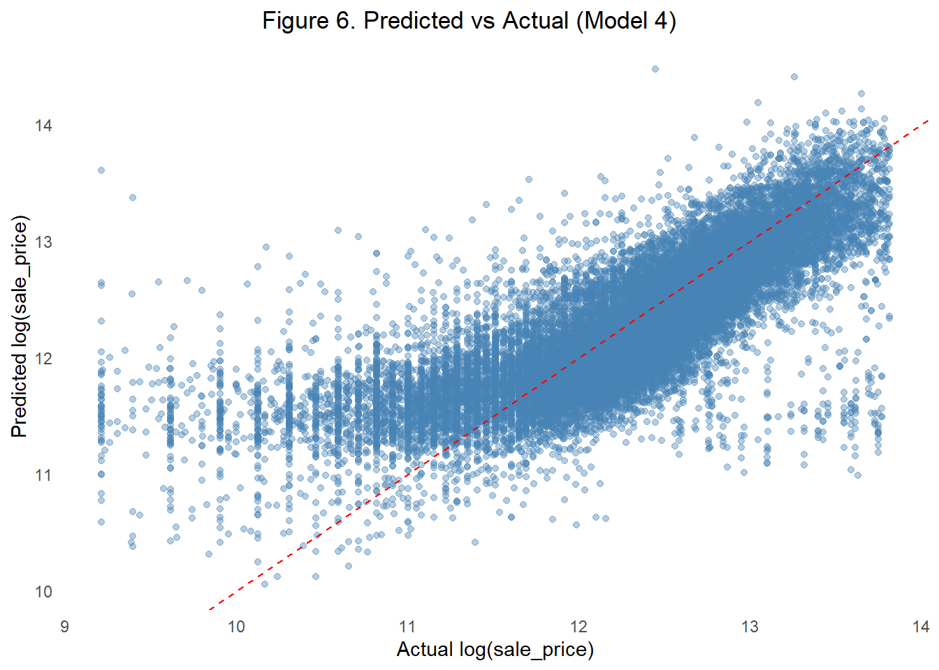
The graph of the actual logged sale prices by the predicted logged sale prices compliments our model performance metrics found in Table 6 as points cluster closely around the reference line suggesting stable consistency in errors and moderate ability to predict sale prices.
Phase 6: Model Diagnostics
When using linear regression to model relationships, we assume a number of conditions are met to support the validity of using a linear model. Here we test various linear modeling assumptions to determine the appropriateness of our model.
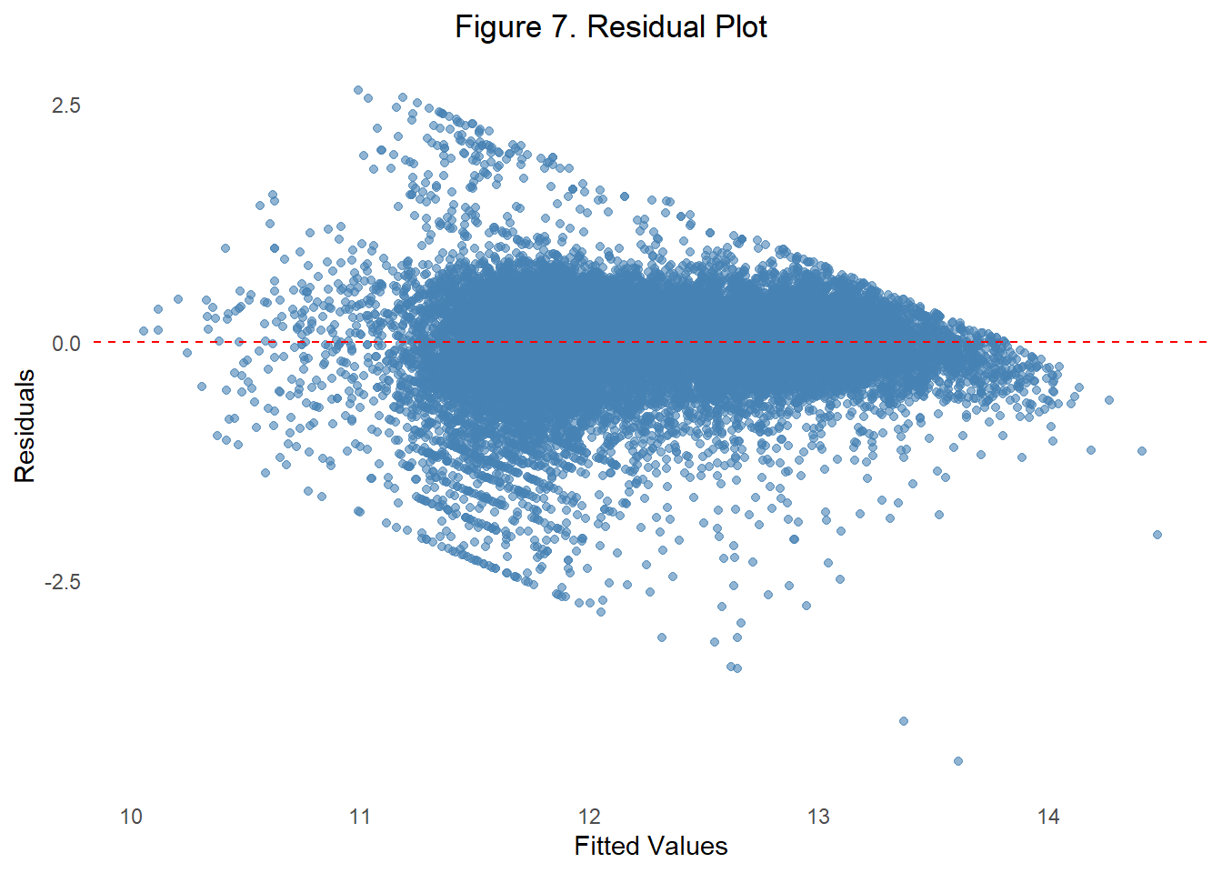
One linear model assumption is the assumption that the relationship is actually linear. If the linearity assumption is met, residuals should be randomly scattered around the zero line with no discernible pattern.
In Figure 7, we plotted the residuals or prediction errors by the model’s fitted values. The red dashed line at zero marks where residuals would fall if predictions were perfect. In this plot, the residuals appear to fan out as fitted values increase, suggesting a possible violation of the linearity. This pattern may indicate that the model under- or over-predicts at different price levels.
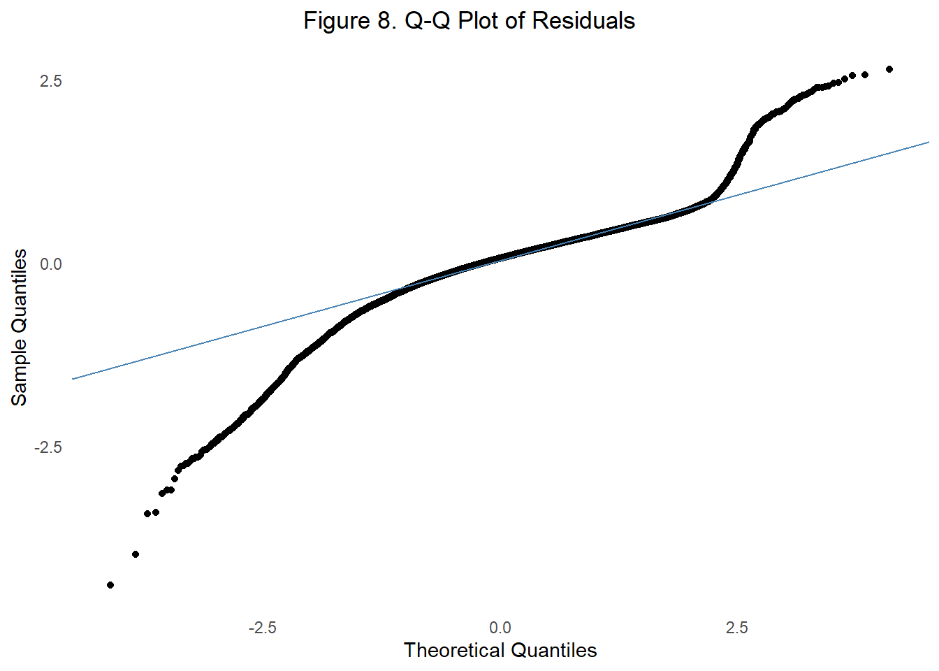
Another assumption we test is the normal distribution of residuals or errors. In Figure 8, we test the assumption of normally distributed residuals using a Q-Q plot. If normality of residual’s is met, the sample quantile points should fall roughly along the blue reference line representing theoretical quantiles of normal distribution.
In this plot, the residuals deviate from the line, particularly in the tails at low and high values, indicating non-normality.
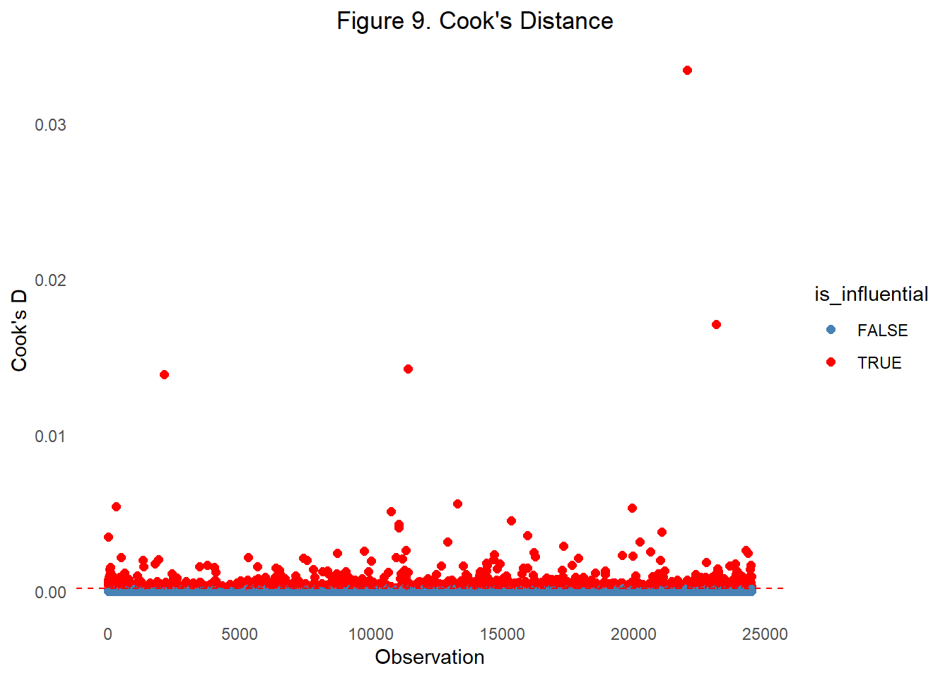
One last regression assumption check we performed was determining whether there were influential outliers present. Figure 9 displays Cook’s Distance values for each observation, with colors indicating whether the point is flagged as influential, blue being none influential observations and red being the influential obeservations. A substantial large number of our observations were marked as influential, suggesting that many data points have both high leverage and large residuals.
Phase 7: Conclusions & Recommendations
The final model demonstrates strong performance, achieving an adjusted R² of 0.591 and explaining nearly 59% of the variation in housing prices across Philadelphia. This marks a substantial improvement over the baseline structural model (Model 1, R² = 0.35), highlighting the value of incorporating spatial characteristics alongside structural and socioeconomic factors.
Among all predictors, total livable area emerges as the most influential driver of price, followed by the number of bathrooms and garage spaces. Exterior condition, median income, and educational attainment also show positive associations. Conversely, poverty rate and local crime density are negatively associated with price.
The interaction between living area and wealthy neighborhoods reveal that additional square footage may not have as much of an impact on price in high-value areas. Spatial dependencies are also evident in the model’s predictive accuracy as prediction errors show spatial patterns. The model performs best in mid-range price neighborhoods but struggles in areas like Nicetown, Fairhill, and Upper Kensington, where residual errors are higher. These disparities raise important equity concerns in the context of policy as these areas that are predisposed to under-prediction in modeling are also historical disadvantaged neighborhoods.
-1.png)