In the NFIRS (National Fire Incident Reporting System) reporting system, false alarms (codes 700–799) include system malfunctions, unintentional activations, detector errors, and malicious alarms. Although no actual fire is present, each false alarm still triggers a full fire department response.
In OpenDataPhilly dataset, 77% of all fire-related incidents are false alarms. This extremely high share creates substantial operational burden: every response requires multiple firefighters, apparatus deployment, fuel and equipment usage, and temporarily removes units from availability for real emergencies.
Reducing false alarms can save time, reduce firefighter workload, and improve public safety. This analysis produces a predicted probability of false alarm for each incident.
By choosing an appropriate threshold, the city can identify high-risk cases and apply targeted interventions to reduce unnecessary responses and operational costs.
2 Data Preparation
2.1 Setup
Code
# Core packageslibrary(tidyverse) # dplyr, ggplot2, readr, tidyr, stringr, etc.library(sf)library(tigris)library(tidycensus)# Modeling / utilitieslibrary(MASS)library(caret)library(broom)library(patchwork)library(scales)library(knitr)library(riem)library(dplyr)library(pROC)library(tidyr)library(lubridate)# tigris optionsoptions(tigris_use_cache =TRUE, tigris_class ="sf", tigris_progress =FALSE)# set a global themetheme_set(theme_minimal(base_size =12))
2.2 Data Import & Cleaning
2.2.1 Fire Incident Data
We recoded incident types following NFIRS conventions. All 7xx incidents represent False Alarm & False Call responses (e.g., alarm system malfunctions, detector errors, accidental activations, and malicious alarms) and were coded as 1. Incidents in the 1xx and 2xx series correspond to actual fires and overpressure/explosion events that required genuine emergency response; these were coded as 0. This classification provides a clean separation between false alarms and all non–false alarm incidents for modeling purposes.
We retrieved tract-level demographic and socioeconomic indicators from the 2023 American Community Survey (ACS) to incorporate neighborhood characteristics that may influence false-alarm patterns. Prior research shows that alarm activity often correlates with community demographics, housing conditions, and economic stressors. Accordingly, we included measures of population composition, educational attainment, income, and labor force status to capture these broader social determinants.
Building certification information comes from the City of Philadelphia’s Licenses and Inspections (L&I) Building Certifications dataset on OpenDataPhilly. We joined these records to the building footprints to identify each building’s fire-alarm certification status (Active, Expired, or Deficient). Including this information allows the model to account for building-level inspection and maintenance conditions, which are closely related to false-alarm occurrences.
  fire_alarm_status     n
1            Active 13241
2           Expired  7635
3              <NA>  5098
4         Deficient   340
We spatially joined the building certification records to census tracts to summarize inspection conditions at the neighborhood level. For each tract, we calculated the number of buildings with Active, Expired, or Deficient fire-alarm certifications and derived an active certification rate. These tract-level indicators were then merged into the ACS dataset, allowing the model to incorporate variation in building inspection status across neighborhoods.
We obtained hourly weather observations from the PHL airport weather station using the riem_measures API. Data were downloaded in several date ranges and combined into a single dataset, from which duplicate timestamps were removed. Including weather information allows the model to capture environmental conditions such as temperature, precipitation, and wind speed that may influence alarm activations and false-alarm likelihood.
From the cleaned weather dataset, we generated a day-of-week variable and an is_weekend flag to capture weekly temporal patterns in alarm activity. Weekend versus weekday distinctions are included because building use and human activity differ substantially across the week. On weekends, many commercial and institutional buildings operate at reduced occupancy, while residential buildings experience increased activity. These shifts can influence how alarm systems behave through factors such as maintenance schedules, system testing times, building vacancy, cooking activity, or nuisance triggers.
# A tibble: 2 × 2
  is_weekend     n
       <int> <int>
1          0   460
2          1   184
2.2.6 Location of Fire Stations
We incorporated the locations of Philadelphia fire stations by converting the Fire_Dept table into a spatial dataset using station latitude and longitude. A 100-meter buffer was generated around each station to capture buildings located very close to fire infrastructure. Proximity to a fire station may relate to false-alarm activity, for example, areas near stations may include larger commercial buildings with more alarm systems, more frequent maintenance activity, or higher reporting sensitivity.
2.3 Data Merge
Multiple contextual variables were merged onto the incident dataset to create a comprehensive analytic file. Weather observations were linked by date, fire station buffers were used to generate a proximity indicator, and incidents were spatially joined to census tracts to attach neighborhood socioeconomic and building-inspection attributes. We also derived temporal structure by assigning each incident to a calendar quarter, and calculated the distance from each incident to Philadelphia City Hall as a simple measure of urban centrality. Together, these additions introduce temporal, spatial, and neighborhood-level variation that may influence false-alarm patterns.
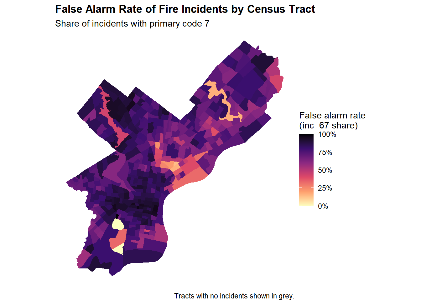
tract_fire_stats <- fire_firetract |>st_drop_geometry() |>dplyr::filter(!is.na(GEOID)) |>dplyr::group_by(GEOID) |>dplyr::summarise(n_incidents = dplyr::n(),n_false_7 =sum(inc_new ==1, na.rm =TRUE),false_rate_7 = n_false_7 / n_incidents)philly_census_alarm_fire <- philly_census_alarm |>dplyr::left_join(tract_fire_stats, by ="GEOID")ggplot(philly_census_alarm_fire) +geom_sf(aes(fill = false_rate_7), color =NA) +scale_fill_viridis_c(option ="magma",direction =-1,na.value ="grey90",labels = scales::percent_format(accuracy =1),name ="False alarm rate\n(inc_67 share)" ) +labs(title ="False Alarm Rate of Fire Incidents by Census Tract",subtitle ="Share of incidents with primary code 7",caption ="Tracts with no incidents shown in grey." ) +theme_void() +theme(legend.position ="right",plot.title =element_text(face ="bold") )
Interpretation
This map shows the spatial distribution of false alarms across Philadelphia census tracts. Each tract is shaded according to the share of incidents classified as false alarms (primary code 7). Darker purple areas represent neighborhoods where false alarms make up a larger proportion of fire responses, while lighter areas exhibit lower false-alarm activity. Tracts with no recorded incidents during the study period are shown in grey. The pattern highlights substantial geographic variation: several central and high-density neighborhoods display elevated false-alarm rates, whereas some peripheral areas show relatively fewer false responses.
3.2 Pie Chart: True Fire vs False Alarm
Code
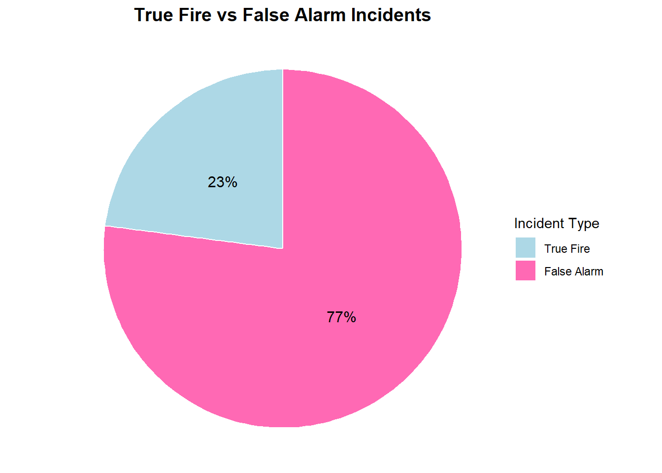
ggplot(binary_summary, aes(x ="", y = p, fill = fire_type)) +geom_col(width =1, color ="white") +geom_text(aes(label = p_label),position =position_stack(vjust =0.5),size =4 ) +coord_polar(theta ="y") +scale_fill_manual(values =c("True Fire"="lightblue","False Alarm"="hotpink" ) ) +labs(title ="True Fire vs False Alarm Incidents",fill ="Incident Type" ) +theme_void() +theme(plot.title =element_text(hjust =0.5,size =14,face ="bold" ) )
Interpretation
The pie chart summarizes the composition of all fire-related incidents in Philadelphia during the study period. False alarms account for 77% of all dispatches, while true fire events represent only 23%. This large imbalance highlights a central operational challenge for the Fire Department: the vast majority of responses do not involve an actual fire, yet still require staff time, equipment movement, and system capacity. The high prevalence of false alarms underscores the importance of predictive modeling to help identify where and when such calls are most likely to occur.
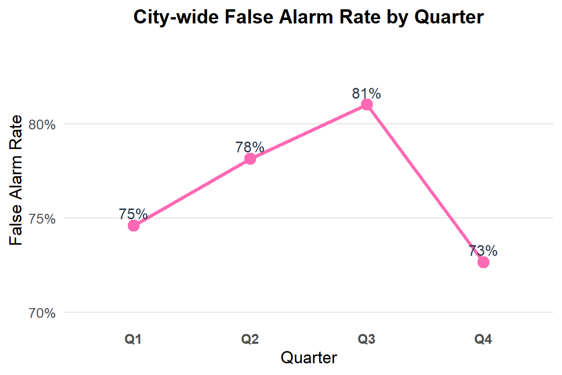
The quarterly trend shows modest but consistent seasonal variation in Philadelphia’s false alarm rate. Rates rise from 75% in Q1 to a peak of 81% in Q3, before dropping to 73% in Q4. This pattern suggests that false alarms become slightly more common during the summer months and decline toward the end of the year. Although the seasonal differences are not dramatic, they highlight that false alarm activity is not evenly distributed across the calendar, which may have implications for staffing, resource planning, and inspection scheduling.
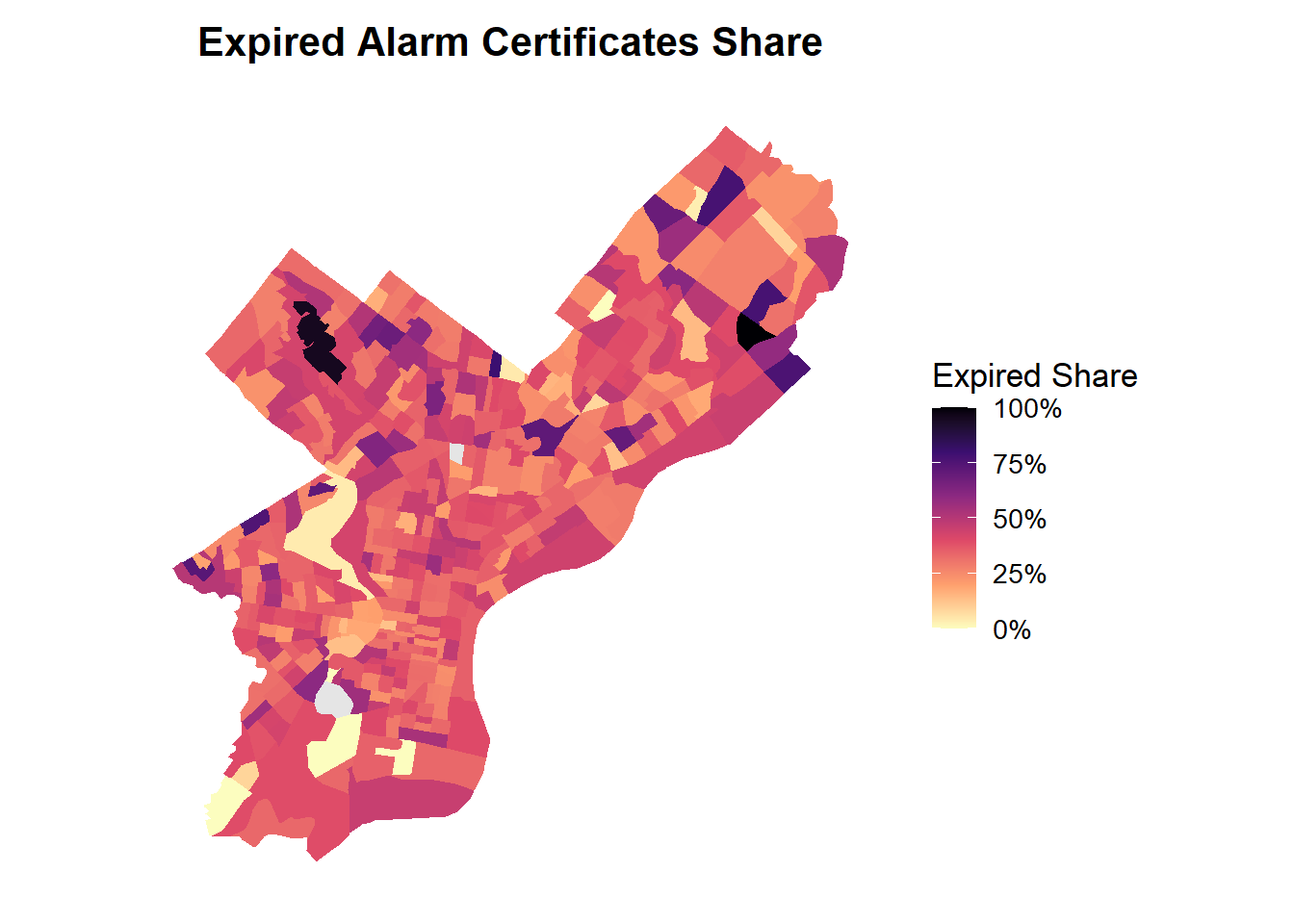
3.4 Map: Expired Alarm Certificates Share by Census Tract
This map illustrates the share of buildings with expired fire alarm certifications across Philadelphia census tracts. Higher-expiry areas (shaded in darker purple) appear in several parts of North and West Philadelphia, as well as pockets of the Northeast. These neighborhoods tend to show a larger proportion of buildings whose annual alarm inspections are overdue, signaling potential maintenance challenges or compliance gaps. In contrast, many tracts in Center City and portions of South Philadelphia display lower expired shares, suggesting stronger inspection adherence. The geographic pattern indicates that certification compliance is not uniform across the city and may align with broader socioeconomic differences, telling us areas where targeted outreach or enforcement may be most needed.
4 Modeling
4.1 Model1: Weather Data
Model 1 is a baseline logistic regression that predicts whether an incident is a false alarm (inc_new = 1) using only weather conditions and building-level activity rates on the day of the call. The model includes:
Temperature: Daily average temperature
Precipitation: Total daily precipitation
Wind_Speed: Average daily wind speed
active_rate: Share of buildings in the tract with an active (valid) fire alarm certification
Logistic Regression Model: Weather Predictors Only
Variable
Estimate
Std. Error
z value
Pr(>|z|)
(Intercept)
0.5846
0.0536
10.91
0.000000
Temperature
0.0101
0.0005
18.64
0.000000
Precipitation
18.5156
5.0734
3.65
0.000263
Wind_Speed
0.0034
0.0023
1.44
0.151000
active_rate
0.1182
0.0810
1.46
0.145000
Logit Model 1 serves as the baseline specification, incorporating only weather variables and the building-level alarm compliance rate to predict whether an incident is a false alarm. The model’s estimates indicate statistically significant effects for temperature and precipitation, suggesting that warmer days and days with measurable precipitation are associated with a higher likelihood of false alarms. In contrast, wind speed and the active certification rate do not reach conventional significance levels in this simplified model. Overall model fit is modest, with limited explanatory power relative to later specifications that incorporate socioeconomic, spatial, and temporal predictors. As expected for a parsimonious model, it captures only a small share of the variation in incident outcomes and primarily functions as a reference point against which the performance gains of more complete models can be assessed.
4.2 Model 2: Socioeconomic
Model 2 extends the baseline specification by incorporating census tract–level socioeconomic characteristics to capture structural factors that may influence false alarm patterns. In addition to the weather variables and active building certification rates from Model 1, this model includes:
median_income: Median household income, reflecting economic resources and potential differences in building conditions. 232qq
ba_rate: Share of adults holding a bachelor’s degree, used as a proxy for neighborhood socio-demographic composition.
black_share: Percentage of Black residents in the tract, capturing racial composition patterns relevant for equity analysis.
unemployment_rate: Local unemployment levels, which may correlate with neighborhood stressors or reporting behaviors.
These variables allow the model to account for broader socioeconomic context rather than relying solely on incident-day environmental factors.
Model 2 expands the baseline specification by incorporating socioeconomic characteristics of each census tract, and its performance improves substantially relative to Model 1. Education level (ba_rate), Black population share, and median income are highly statistically significant, indicating that false alarm patterns are strongly associated with underlying demographic and socioeconomic conditions. The model’s coefficients suggest that areas with higher educational attainment and larger Black population shares exhibit higher probabilities of false alarms, even after controlling for weather and building-level compliance activity. Compared with the baseline model, the residual deviance decreases from 67133 to 59730 and the AIC drops from 67143 to 59748, indicating a markedly better fit. These gains show that socioeconomic context meaningfully contributes to predicting false alarms and helps explain variation that weather alone cannot.
4.3 Model 3: Full Model
Model 3 extends the previous specifications by incorporating temporal patterns and spatial accessibility factors that may influence the likelihood of a false alarm. In addition to weather, building characteristics, and neighborhood socioeconomic indicators, this model includes:
is_weekend : Whether the incident occurred on a weekend, capturing changes in occupancy, human activity, and reporting behavior between weekdays and weekends.
quarter: A categorical indicator for seasonal variation (Q1–Q4), allowing the model to account for cyclical patterns in alarm activity across the year.
near_station_200m: A binary variable identifying incidents that occur within 200 meters of a fire station, representing potential differences in response environments and built-environment characteristics around stations.
dist_cityhall_km: The distance from the incident location to Philadelphia City Hall, serving as a proxy for urban centrality and potential differences between high-density downtown areas and more peripheral neighborhoods.
The full model delivers the strongest predictive performance among the three specifications. Adding socioeconomic factors, temporal indicators, and spatial proximity variables substantially improves model fit, reducing deviance and lowering AIC compared to Models 1 and 2. Several predictors show significant associations with false-alarm likelihood, most notably education level, racial composition, unemployment rate, and building certification activity while weather variables retain moderate predictive power. Temporal effects are modest but present, with higher false-alarm rates in Q3 and lower rates in Q4. Spatial features contribute additional explanatory value, as calls nearer to fire stations and farther from Center City are slightly less likely to be false alarms. Overall, the full model captures the most complete set of behavioral, environmental, and geographic signals and therefore serves as the best-performing specification for subsequent interpretation and policy analysis.
4.4 Model Evaluation
4.4.1 AUC Comparison
Code
dat1 <-model.frame(logit_model1) p1 <-predict(logit_model1, type ="response")roc1 <-roc(dat1$inc_new, p1)auc1 <-auc(roc1)dat2 <-model.frame(logit_model2)p2 <-predict(logit_model2, type ="response")roc2 <-roc(dat2$inc_new, p2)auc2 <-auc(roc2)dat3 <-model.frame(logit_model3)p3 <-predict(logit_model3, type ="response")roc3 <-roc(dat3$inc_new, p3)auc3 <-auc(roc3)data.frame(model =c("logit_model1", "logit_model2", "logit_model3"),AUC =c(auc1, auc2, auc3))
Across the three logistic regression specifications, predictive performance improves steadily as additional structural, socioeconomic, and temporal features are introduced. Model 1 achieves an AUC of 0.554, indicating very limited predictive power and only marginal improvement over random guessing. Adding socioeconomic variables in Model 2 substantially increases the AUC to 0.670, suggesting that neighborhood‐level demographic and income patterns provide meaningful signal in distinguishing false alarms from true fire events. The full model (Model 3), which incorporates temporal indicators, proximity to fire stations, and distance to downtown, yields the highest AUC of 0.672. Although the improvement over Model 2 is modest, it indicates that these operational and spatial predictors add incremental information beyond weather and socioeconomic structure.
4.4.2 ROC Curve
Code
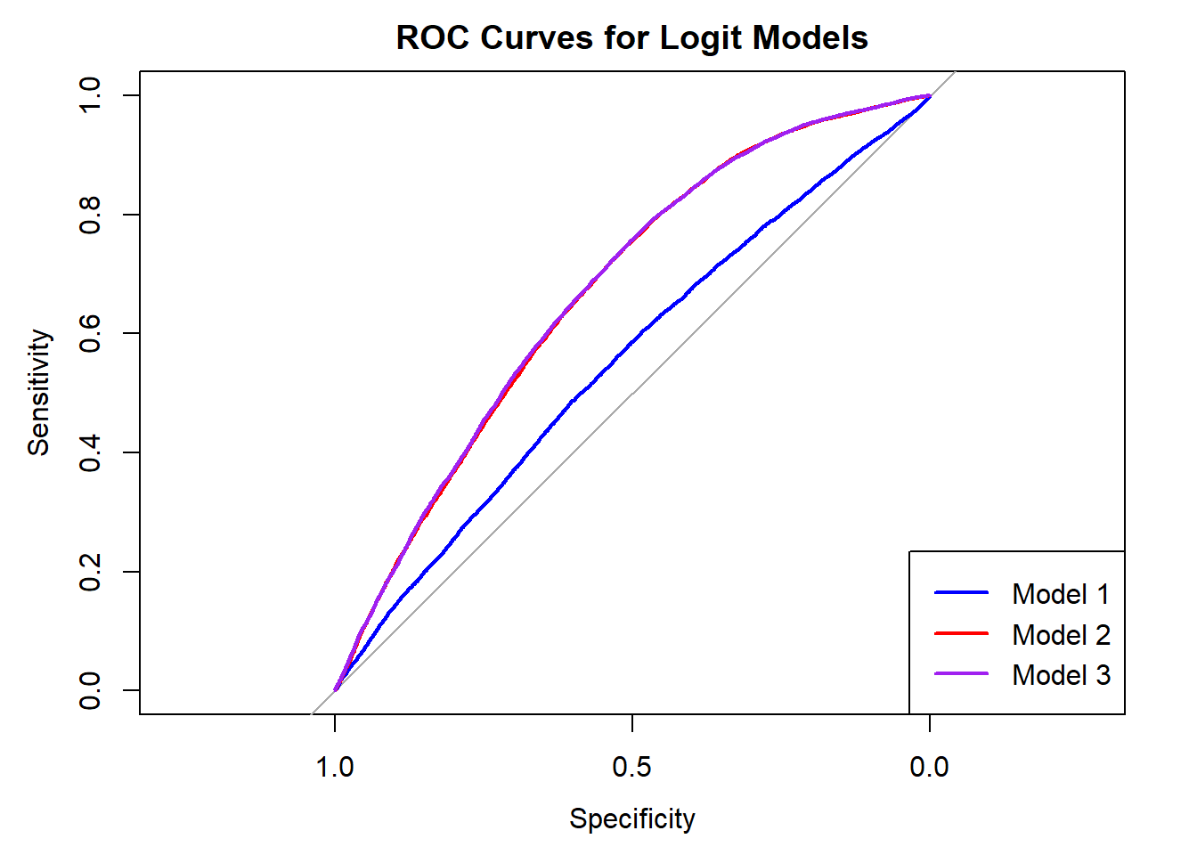
plot(roc1, col ="blue", lwd =2, main ="ROC Curves for Logit Models")plot(roc2, col ="red", lwd =2, add =TRUE)plot(roc3, col ="purple", lwd =2, add =TRUE)legend("bottomright",legend =c("Model 1", "Model 2", "Model 3"),col =c("blue", "red", "purple"),lwd =2)
The ROC curves visualize how each model balances sensitivity and specificity across all possible thresholds. Model 1 shows the weakest discrimination, with a curve only slightly above the 45-degree no-skill line. Model 2 improves substantially once socioeconomic characteristics are added, producing a visibly steeper curve. Model 3 offers a modest gain: adding temporal factors and spatial proximity variables produces the strongest curve overall, indicating the most consistent ability to distinguish false alarms from real incidents across thresholds.
Generalized Linear Model

59340 samples
   12 predictor
    2 classes: 'FalseAlarm', 'RealIncident'

No pre-processing
Resampling: Cross-Validated (5 fold)
Summary of sample sizes: 47472, 47473, 47471, 47472, 47472
Resampling results:

  ROC       Sens       Spec
  0.671565  0.9858302  0.06613265
To assess the stability of the full logistic regression model, we conduct 5-fold cross-validation on the training data. The cross-validated ROC (0.672) is nearly identical to the in-sample ROC reported earlier, indicating that the model’s predictive performance is highly stable across different data splits. The very high sensitivity and low specificity largely reflect the substantial class imbalance in the outcome (false alarms ≈ 77%). Because classification thresholds are not yet optimized at this stage, these values are not used for model selection; instead, cross-validation primarily confirms that the model generalizes consistently.
The odds‐ratio table summarizes how each predictor influences the likelihood that an incident is classified as a false alarm after controlling for all other variables. Weather variables, particularly temperature and precipitation, remain strong predictors, with higher temperatures and any measurable precipitation increasing the likelihood of a false alarm. Building compliance also matters: tracts with higher active certification rates show significantly greater odds of false alarms, consistent with patterns observed in the earlier models. Socioeconomic context continues to contribute meaningful signal, higher educational attainment, a larger Black population share, and higher unemployment are all associated with elevated false-alarm odds, even after controlling for weather and temporal factors. Temporal features add smaller but still interpretable effects: false alarms are slightly less likely on weekends and in Q4, and marginally more likely in Q3. Finally, spatial accessibility plays a role: incidents occurring near a fire station (<200m) or farther from Center City show modestly reduced odds of being false alarms. Together, these results suggest that false-alarm activity reflects an interaction of environmental conditions, neighborhood characteristics, and system operations.
4.5 Threshold Selection
In a logistic regression model, predicted values represent the probability that an incident is a false alarm. To convert these probabilities into binary classifications (false alarm vs. real incident), a decision threshold must be chosen. Different thresholds produce different trade-offs between sensitivity (true positive rate) and specificity (true negative rate).
We evaluated two candidate thresholds—0.9 and 0.4—to illustrate how classification behavior changes under different risk tolerances.
Threshold = 0.9 (Conservative) A threshold of 0.9 classifies an incident as a false alarm only when the predicted probability is extremely high.
Very high specificity (96.4%): almost all true incidents are correctly labeled as real.
Very low sensitivity (8.1%): the model fails to identify most false alarms (42,024 false negatives).
This threshold minimizes false positives but misses the vast majority of false alarms. This setting is appropriate in contexts where misclassifying a real emergency as a false alarm is unacceptable, such as prioritizing safety or enforcement on only the most extreme cases.
Threshold = 0.4 (Aggressive) A threshold of 0.4 classifies an incident as a false alarm when the predicted probability exceeds 40%.
Extremely high sensitivity (99.95%): nearly all false alarms are detected (only 23 missed).
Very low specificity (0.28%): almost all true incidents are incorrectly labeled as false alarms.
This threshold identifies almost every false alarm but also generates a large number of false positives. This setting is useful in contexts where the goal is to maximize detection, such as broad preventive inspections or outreach.
5 Recommendations
Threshold should be chosen based on capacity and goals. Based on the model comparison and operational needs, we recommend adopting a relatively aggressive threshold as the decision rule to catch more possible false alarms. Selecting a lower threshold does not imply that the Fire Department will ignore these calls; rather, it allows the Department to differentiate levels of risk more effectively. When the model indicates a high likelihood of a false alarm, fire crews would still respond, but they can deploy a lighter response package, smaller teams, fewer apparatus, and reduced resource commitment. This minimizes unnecessary operational costs, reduces roadway risk, and preserves capacity for true emergencies. In addition, for calls predicted as likely false alarms, response teams can carry educational materials, communication guidelines, and basic fire-alarm inspection toolkits, allowing them to both address the call and engage with property managers about system maintenance and common causes of false activations.
Beyond operational adjustments, we also recommend a set of longer-term policy strategies.
First, the City should strengthen mandatory fire-alarm inspection and compliance enforcement. For buildings with repeated false alarms or expired certificates, a tiered penalty structure or more frequent re-inspections may create stronger incentives for timely system maintenance.
Second, the City should expand public and community education efforts. The Fire Department could host workshops, property-manager trainings, or community sessions on alarm maintenance, common malfunction causes, and mitigation strategies. Targeted outreach may be especially effective in neighborhoods or buildings with historically high false-alarm rates.
6 Limitations&Next Steps
6.1Limitations
Although the model provides meaningful predictive ability, it still faces several important limitations. First, the data contain gaps and inconsistencies, for example, missing or outdated fire-alarm certificate records and uneven data quality across neighborhoods which can reduce model stability. Second, because the current model is binary, it can only classify alarms as “false” vs. “not false,” and cannot distinguish different levels of fire risk. No matter how high or low the predicted probability is, the final decision still requires using a single threshold, which restricts how much nuance the model can express. In addition, any misclassification carries real consequences: mislabeling a true fire as a false alarm could delay response, while treating a likely false alarm as high risk may burden residents and property owners and potentially exacerbate existing enforcement inequities. For these reasons, the model should be used as a decision-support tool rather than a substitute for professional judgment.
6.2Improvement Possibilities
With richer data, more development time, or additional funding, the model could be expanded into a multi-tier risk classification system, instead of a simple binary prediction. For example, alarms could be grouped into four levels:
Tier 1 = high emergency (very likely real fire)
Tier 2 = moderate risk (standard response)
Tier 3 = minor risk (non-emergency conditions possible)
Achieving this would require integrating additional features, such as alarm device age, building maintenance histories, humidity/smoke environment data, renovation activity, and more granular spatial patterns. These richer inputs would allow the model to shift from hard thresholding to continuous risk scoring and tiered operational strategies, enabling more precise allocation of fire-department resources. Future enhancements could also include multiclass models or time-series analysis to support an even more nuanced and safety-balanced dispatch framework.