Philadelphia Housing Model—Technical Appendix

Predicting Residential Property Prices

Data Cleaning

Primary Philadelphia Sales Data (OpenDataPhilly)

# Import relevant libraries.
library(car)
library(dplyr)
library(ggcorrplot)
library(ggplot2)
library(grid)
library(gridExtra)
library(knitr)
library(kableExtra)
library(scales)
library(sf)
library(stringr)
library(tibble)
library(tidycensus)
library(tidyr)
library(tidyverse)
library(tigris)
library(tmap)
library(units)

options(scipen = 999)

# Property data.
properties_path <- "data/philly_properties.csv"
properties <- read.csv(properties_path)

# Capture dimensions.
og_property_dimension <- dim(properties)

# Set Census API key.
census_api_key("3aaee31789e10b674a531e9f236c35d5394b19ed")

# All variables are character strings, remove white space then convert numeric character variables to numeric classes for chosen variables.

properties <- properties %>%
  mutate(across(where(is.character), str_trim),
         across(c(fireplaces, garage_spaces, number_of_bathrooms, number_stories,
                  sale_price, total_livable_area, year_built), as.numeric)) %>%
  rename(fireplace_num = fireplaces,
         garage_num = garage_spaces,
         bath_num = number_of_bathrooms,
         story_num = number_stories,
         square_feet = total_livable_area,
         basement_type = basements,
         ac_binary = central_air,
         fuel_type = fuel,
         )

# Filter to residential properties and 2023-2024 sales.
# Note: Category code #1 is for residential.
residential_prop <- properties %>%
  filter(.,
         category_code == 1,
         startsWith(sale_date, "2023") | startsWith(sale_date, "2024"))

# Drop empty variables or variables not needed for model.
residential_prop <- residential_prop %>%
  select(c(basement_type, ac_binary, fireplace_num, fuel_type, garage_num,
           bath_num, story_num, sale_date, sale_price,
           square_feet, year_built, shape)
         )

# Make empty character column values NA.
residential_prop <- residential_prop %>%
  mutate(across(where(is.character), ~na_if(., "")))

# Drop prices that are less than $10,000 as a catch-all (might not be as reflective for rural areas). Avoiding dropping prices based on percent of assessed value since property assessments can be biased against minoritized communities. Ideal drop would add deed type to drop any family or forced transfers.
residential_prop <- residential_prop %>%
  filter(sale_price > 10000,
         square_feet > 0) %>%
  mutate(.,
         price_per_sqft = sale_price / square_feet) %>%
  filter(.,
         price_per_sqft > quantile(price_per_sqft, 0.05, na.rm = TRUE))

# Create building age column, change central air to binary, and adjust basement and fuel types.
# Create log value for the sale price.
residential_prop <- residential_prop %>%
  mutate(ln_sale_price = log(sale_price),
         age = 2025 - year_built,
         ln_square_feet = log(square_feet),
         ac_binary = case_when(
           ac_binary == "Y" ~ 1,
           ac_binary == "N" ~ 0),
         basement_type = case_when(
           basement_type == "0" ~ "None",
           basement_type == "A" ~ "Full Finished",
           basement_type == "B" ~ "Full Semi-Finished",
           basement_type == "C" ~ "Full Unfinished",
           basement_type == "D" ~ "Full Unknown Finish",
           basement_type == "E" ~ "Partial Finished",
           basement_type == "F" ~ "Partial Semi-Finished",
           basement_type == "G" ~ "Partial Unfinished",
           basement_type == "H" ~ "Partial Unknown Finish",
           basement_type == "I" ~ "Unknown Size Finished",
           basement_type == "J" ~ "Unknown Size Unfinished"),
         fuel_type = case_when(
           fuel_type == "A" ~ "Natural Gas",
           fuel_type == "B" ~ "Oil Heat",
           fuel_type == "C" ~ "Electric",
           fuel_type == "D" ~ "Coal",
           fuel_type == "E" ~ "Solar",
           fuel_type == "F" ~ "Wood",
           fuel_type == "G" ~ "Other",
           fuel_type == "H" ~ "None")
         )

# Turn categorical data into factors so OLS regression doesn't handle the data as a list of strings.
residential_prop$basement_type <- as.factor(residential_prop$basement_type)
residential_prop$fuel_type <- as.factor(residential_prop$fuel_type)

# Change the reference categories for baseline comparison.
residential_prop$basement_type <- relevel(residential_prop$basement_type, ref = "None")
residential_prop$fuel_type <- relevel(residential_prop$fuel_type, ref = "Natural Gas")

# Place fuel type with 10 or less counts into other category.
residential_prop <- residential_prop %>%
  mutate(fuel_type = fct_lump_min(fuel_type, min = 11, other_level = "Other"))

# Fixed effect temporal market fluctuations. Based on sale date, splitting the years into quarters (Q1, Q2, Q3, Q4). Potential fixed effect.
residential_prop <- residential_prop %>%
  mutate(
    quarters_fe = quarter(as_datetime(sale_date))
    )

# Make it a factor.
residential_prop$quarters_fe <- factor(residential_prop$quarters_fe)

# Capture dimensions.
after_property_dimension <- dim(residential_prop)

# Convert residential property to geodataframe. Use EPSG 2272 for South Pennsylvania in feet.
# Drop shape when finished creating geometry.
residential_prop_gdf <- residential_prop %>%
  mutate(geometry = st_as_sfc(shape)) %>%
  st_as_sf(crs = 2272) %>%
  rename(geometry_point = geometry) %>%
  select(-c(shape))

Spatial Data and Feature Engineering

Spatial Data (OpenDataPhilly)

# Read in Philadelpha census tracts.
philly_tracts_path <- "data/philly_tracts/philly_tracts.shp"
philly_tracts <- st_read(philly_tracts_path)

Reading layer `philly_tracts' from data source 
  `C:\Users\Tess\Documents\GitHub\portfolio-setup-TessaVu\midterm-project\data\philly_tracts\philly_tracts.shp' 
  using driver `ESRI Shapefile'
Simple feature collection with 3446 features and 12 fields
Geometry type: MULTIPOLYGON
Dimension:     XY
Bounding box:  xmin: -80.51985 ymin: 39.7198 xmax: -74.68956 ymax: 42.51607
Geodetic CRS:  NAD83

# Match CRS.
philly_tracts <- st_transform(philly_tracts, crs = 2272)

# Left spatial join.
residential_points <- st_join(residential_prop_gdf, philly_tracts)

# Drop unnecessary columns and remove incomplete observations (rows) for upcoming spatial feature computations.
residential_points <- residential_points %>%
  select(-c(FUNCSTAT, MTFCC, NAMELSAD, NAME,
            STATEFP, COUNTYFP, TRACTCE)) %>%
  na.omit(.)

# Remove unneeded datasets for housekeeping and call garbage collector to reduce memory.
rm(properties, residential_prop, residential_prop_gdf)
gc()

           used  (Mb) gc trigger   (Mb)  max used   (Mb)
Ncells  8660780 462.6   12563275  671.0  11778460  629.1
Vcells 73531134 561.0  138446873 1056.3 138446681 1056.3

# Proximity to downtown.

# Decided on Euclidean distance because network proximity computation is demanding on thousands of points, even with parallel programming.

# Create single Center City point feature based on City Hall coordinates.
center_city <- st_sfc(st_point(c(-75.163500, 39.952800)), crs = 4326) %>%
  st_transform(crs = 2272)

# Need to add mile units for operations. Then remove units object for easier plotting.
residential_points$city_dist_mi <- (st_distance(residential_points, st_union(center_city))) %>%
  set_units("mi") %>%
  drop_units() %>%
  as.numeric()

# Log transform because distance benefit diminishes, for potential use.
residential_points$ln_city_dist <- log(residential_points$city_dist_mi + 0.1)

# Transit proximity.
# Major cities could be distance to nearest transit like metro/rail stations, but suburban and rural areas might be better served by distance to nearest major highway.
# Read in SEPTA stops.
septa_stops_path <- "data/septa_stops.csv"

septa_stops_df <- read.csv(septa_stops_path)

# Make csv a geodataframe.
septa_stops <- septa_stops_df %>%
  st_as_sf(., coords = c("Lon", "Lat"), crs = 4326)

# Match CRS.
septa_stops <- septa_stops %>%
  st_transform(., crs = 2272)

# Stops are duplicated for the same station because the data includes directions for all cardinal directions as well as bus, rail, and trolley for the same location. This means a single station could have more than one point representing a single location residents go to commute.
# Create new column with stop name without the cardinal suffixes and keep only the unique station values.
septa_stops <- septa_stops %>%
  mutate(stations = if_else(
    str_detect(StopAbbr, "NO$|SO$|EA$|WE$|NE$|NW$|SE$|SW$"),
    str_sub(StopAbbr, end = -3),
    str_sub(StopAbbr)
    )
  ) %>%
  distinct(stations, .keep_all = TRUE)

# Create buffer zone for stops within a half mile. This is ~10 minute walk, depending on topography.
# Note: EPSG 2272 is measured in feet, not miles.
septa_distance <- st_buffer(residential_points, 2640)

# Create number of stops in the buffer zone.
septa_stations <- st_intersects(septa_distance, septa_stops)

# Append buffer zone counts and put into main tract data. Create a logged version for potential use as well because distance benefit tapers off.
residential_points <- residential_points %>%
  mutate(
    septa_half_mi = lengths(septa_stations),
    ln_septa_half_mi = log(septa_half_mi + 0.1)
  )

# Park proximity / size. Measuring distance is important for accessibility, but the size of the park often matters because a property near a block-sized pocket of green space is not equivalent to being near a large one like Wissahickon Valley Park.

# Read in geojson data.
parks_path <- "data/parks.geojson"

parks <- st_read(parks_path)

Reading layer `parks' from data source 
  `C:\Users\Tess\Documents\GitHub\portfolio-setup-TessaVu\midterm-project\data\parks.geojson' 
  using driver `GeoJSON'
Simple feature collection with 63 features and 18 fields
Geometry type: MULTIPOLYGON
Dimension:     XY
Bounding box:  xmin: -75.2837 ymin: 39.87048 xmax: -74.95865 ymax: 40.13191
Geodetic CRS:  WGS 84

# Match CRS and filter by parks.
parks <- parks %>%
  st_transform(., crs = 2272) %>%
  filter(str_detect(USE_, "PARK"))

# Get distance to the edge of the nearest park.
# Note: Don't try to do spatial operations in apply() and mutate().
# Distance matrix of residential properties to parks.
parks_matrix <- st_distance(residential_points, parks)

# Get the nearest distance for each point.
residential_points$parks_mile <- apply(parks_matrix, 1, min)

# Convert to miles.
residential_points$parks_mile <- as.numeric(residential_points$parks_mile) / 5280

# Log parks data for potential use because of diminishing distance benefits.
residential_points$ln_park_dist <- as.numeric(log(residential_points$parks_mile + 0.1))

# Convenience/Food points of interest. Using kNN to measure the density of these amenities rather than nearest amenity point.
amenities_path <- "data/osm_pois/osm_pois.shp"
amenities <- st_read(amenities_path)

Reading layer `osm_pois' from data source 
  `C:\Users\Tess\Documents\GitHub\portfolio-setup-TessaVu\midterm-project\data\osm_pois\osm_pois.shp' 
  using driver `ESRI Shapefile'
Simple feature collection with 65127 features and 4 fields
Geometry type: POINT
Dimension:     XY
Bounding box:  xmin: -80.52111 ymin: 39.71816 xmax: -74.69473 ymax: 42.25797
Geodetic CRS:  WGS 84

# Filter amenities by convenience and food.
amenities <- amenities %>%
  filter(fclass %in% c(
    "atm", "bakery", "bank", "bar", "beauty_shop", "biergarten", "bookshop",
    "butcher", "cafe", "convenience", "department_store", "fast_food", "food_court",
    "greengrocer", "hairdresser", "kiosk", "laundry", "market_place", "pharmacy",
    "mall", "pub", "restaurant", "supermarket"
  )
         ) %>%
  st_transform(., crs = 2272)

# Distance matrix of residential properties to amenities.
amenities_matrix <- st_distance(residential_points, amenities)

# k-Nearest Neighbors (kNN) function.
knn_distance <- function(distance_matrix, k) {
  apply(distance_matrix, 1, function(distances){
    mean(as.numeric(sort(distances)[1:k]))
  })
}

# Create kNN feature for amenities. k = 4 to balance for urban and suburban areas, probably not as representative of rural areas.
residential_points <- residential_points %>%
  mutate(
    knn_amenity_mi = as.numeric(knn_distance(amenities_matrix, k = 4))
  )

# Convert to miles.
residential_points$knn_amenity_mi <- as.numeric(residential_points$knn_amenity_mi / 5280)

# Fixed effect neighborhoods.
neighborhoods_path <- "data/philadelphia_neighborhoods/philadelphia_neighborhoods.shp"
philly_neighborhoods <- st_read(neighborhoods_path)

Reading layer `philadelphia_neighborhoods' from data source 
  `C:\Users\Tess\Documents\GitHub\portfolio-setup-TessaVu\midterm-project\data\philadelphia_neighborhoods\philadelphia_neighborhoods.shp' 
  using driver `ESRI Shapefile'
Simple feature collection with 159 features and 5 fields
Geometry type: POLYGON
Dimension:     XY
Bounding box:  xmin: -75.28026 ymin: 39.86701 xmax: -74.95576 ymax: 40.13799
Geodetic CRS:  WGS 84

# Match CRS.
philly_neighborhoods <- philly_neighborhoods %>%
  st_transform(., crs = 2272)

# Join to residential points and rename to neighborhoods.
residential_points <- residential_points %>%
  st_join(., philly_neighborhoods) %>%
  rename(neighborhood_fe = MAPNAME)

# Make the neighborhoods a factor.
residential_points$neighborhood_fe <- relevel(factor(residential_points$neighborhood_fe), ref = "East Falls")

# Place neighborhoods with 10 or less sales into a small neighborhoods category.
residential_points <- residential_points %>%
  mutate(neighborhood_fe = fct_lump_min(neighborhood_fe, min = 11, other_level = "Small Neighborhoods"))

# Capture spatial feature dimensions.
after_feat_eng_dimension <- dim(residential_points)

# Spatial feature creation table, select spatial features into a separate data frame and drop geometry.
spatial_feature_df <- residential_points %>%
  select(c(city_dist_mi, ln_city_dist, septa_half_mi, ln_septa_half_mi,
           parks_mile, ln_park_dist, knn_amenity_mi)) %>%
  na.omit(.) %>%
  st_drop_geometry()

# Create a tibble from the selected spatial features.
spatial_summary <- tibble(
  "Spatial Features" = names(spatial_feature_df),
  "Description" = c("Distance from city (mi).", "Log of distance from city.", "Within 0.5mi of SEPTA station.",
                    "Log of 0.5 SEPTA station.", "Distance from nearest park (mi).",
                    "Log of distance from nearest park.", "k-Nearest Neighbors convenience and food amenities.")
)

# Make Kable of spatial features.
spatial_kable <- kable(spatial_summary,
                       caption = "Feature Engineered Variables",
                       format.args = list(big.mark = ",")
) %>%
  kable_styling(latex_options = "striped",
                full_width = FALSE) %>%
  column_spec(1, bold = TRUE, width = "5cm") %>%
  row_spec(0, color = "#f5f4f0", background = "#ff4100", bold = TRUE)

spatial_kable

Feature Engineered Variables

Spatial Features	Description
city_dist_mi	Distance from city (mi).
ln_city_dist	Log of distance from city.
septa_half_mi	Within 0.5mi of SEPTA station.
ln_septa_half_mi	Log of 0.5 SEPTA station.
parks_mile	Distance from nearest park (mi).
ln_park_dist	Log of distance from nearest park.
knn_amenity_mi	k-Nearest Neighbors convenience and food amenities.

Primary:

From the CSV, we are analyzing the conditions of basements, number of fireplaces, garage spaces, number of bathrooms, number of stories, the total livable area in square feet, the existence of central air, and type of fuel used on the property. We filtered residential category code with the sale dates between 2023 and 2024. We eliminated property prices <10k. Rather than adhering to the percentage of assessed value as a guide for this filter, for it could incorporate marginalized bias, filtering the property prices removes non-market transactions but still incorporates a wide diversity of communities.

The forced the central air characteristic to become binary rather than “Y” and “N” and made sure to turn the categorical data to factors. The reference categories for types of basements is “None” and for fuel type, it’s “Natural Gas”. We including a building age category computed from the year built data. We logged the square footage and the sale price to correct for right-skewedness.

Spatial:

We inserted the Philadelphia census tracts, changing the CRS to 2272, the ideal projection for SE Pennsylvania analysis. We decided to perform a log transformation on the following variables - city_dist (distance from City Hall in Center City), septa_half_mi (half mile buffer zone from all septa stops within the city geometry), and parks_dist (distance to edge of nearest park in miles) - because their effects on housing prices were non-linear. This transformation ensures that changes in proximity are measured more consistently across the range of distances, rather than being dominated by properties very close to these features.

Regarding amenities, we used k-NN (k nearest neighbors) to measure the density of amenity accessibility rather than individual point data. The amenities are as follows: ATM, bakery, bank, bar, beauty shop, biergarten, bookshop, butcher, café, convenience, department store, fast food, food court, greengrocer, hairdresser, kiosk, laundry, marketplace, pharmacy, mall, pub, restaurant, supermarket. We filtered by convenience and food, transformed the CRS to 2272 for consistency, and then developed a matrix. The distance was inverted, log-transformed to account for diminishing returns, and scaled it to produce a single numeric value in which higher, positive values indicate greater accessibility to amenities.

We included neighborhoods as fixed effects to help explain unknown, unquantifiable factors like cultural atmosphere and other neighborhood-specific factors we cannot statistically account for that may influence housing prices. It was converted into a factor so each neighborhood can receive its own baseline model. Fiscal quarters were also introduced as fixed effects; splitting a year into 4 quarters for unknown factors when it comes to purchasing property (e.g. people are more likely to buy real estate in spring and summer).

Census Data (TidyCensus)

# Open tidycensus data. Using 2023 data, because we are looking at sales 2023-2024
acs_vars <- load_variables(2023, "acs5", cache = TRUE)

# Get acs dimensions.
og_acs_dimension <- dim(acs_vars)

# The variables that we want from tidycensus
variables <- c(
  median_household_income = "B19013_001",
  total_pop = "B01003_001",
  poverty_white = "B17001A_001", # To get poverty percentage
  poverty_black = "B17001B_001",
  poverty_native = "B17001C_001",
  poverty_asian = "B17001D_001",
  poverty_islander = "B17001E_001",
  poverty_other = "B17001F_001",
  poverty_multiracial = "B17001G_001",
  male_18_24_bach = "B15001_009", # Tracts only show bachelor's degrees, unless we want to look at only people 25+
  male_25_34_bach = "B15001_017",
  male_35_44_bach = "B15001_025",
  male_45_64_bach = "B15001_033",
  male_65plus_bach = "B15001_041",
  female_18_24_bach = "B15001_050",
  female_25_34_bach = "B15001_058",
  female_35_44_bach = "B15001_066",
  female_45_64_bach = "B15001_074",
  female_65plus_bach = "B15001_082",
  total_vacant = "B25005_001", # To get vacancy percentage
  white_total_units = "B25032A_001", # Need total units to get percentage of single, detached units and vacant units.
  white_single_family = "B25032A_002",
  black_total_units = "B25032B_001",
  black_single_family = "B25032B_002",
  native_total_units = "B25032C_001",
  native_single_family = "B25032C_002",
  asian_total_units = "B25032D_001",
  asian_single_family = "B25032D_002",
  islander_total_units = "B25032E_001",
  islander_single_family = "B25032E_002",
  other_total_units = "B25032F_001",
  other_single_family = "B25032F_002",
  multiracial_total_units = "B25032G_001",
  multiracial_single_family = "B25032G_002",
  medhhinc_white = "B19013A_001", # Median Household Income
  medhhinc_black = "B19013B_001",
  medhhinc_native = "B19013C_001", 
  medhhinc_asian = "B19013D_001", 
  medhhinc_other = "B19013F_001",  # There is no tract data for native hawiian/pacific islander, I'm including it with other
  medhhinc_multiracial = "B19013G_001", 
  white_pop = "B01001A_001",
  black_pop = "B01001B_001",
  native_pop = "B01001C_001",
  asian_pop = "B01001D_001",
  islander_pop = "B01001E_001",
  other_pop = "B01001F_001",
  multiracial_pop = "B01001G_001"
)

# We are grouping our data by tracts
philly_tract_acs <- get_acs(
  geography = "tract",
  state = "PA",
  variables = variables,
  year = 2022,
  survey = "acs5",
  cache_table = TRUE, 
  output = "wide"
)

# Summing up the variables that we need to create our percentage variables
philly_tract_acs <- philly_tract_acs %>%
  mutate(
    total_poverty = poverty_whiteE + poverty_blackE + poverty_nativeE + poverty_asianE + poverty_islanderE + poverty_otherE + poverty_multiracialE, # Adding all poverty populations together 
    
    total_bach = male_18_24_bachE + male_25_34_bachE + male_35_44_bachE + male_45_64_bachE + male_65plus_bachE + female_18_24_bachE + female_25_34_bachE + female_35_44_bachE + female_45_64_bachE + female_65plus_bachE, #Adding all bachelors degrees together
    
    total_units = white_total_unitsE + black_total_unitsE + native_total_unitsE + asian_total_unitsE + islander_total_unitsE + other_total_unitsE + multiracial_total_unitsE, # Total housing units
    
    total_single_family = white_single_familyE + black_single_familyE + native_single_familyE + asian_single_familyE + islander_single_familyE + other_single_familyE + multiracial_single_familyE # Total single family homes
  )

# Creating our variables that we are going to analyze
philly_tract_acs <- philly_tract_acs %>%
  mutate(
    pct_poverty = (total_poverty/total_popE)*100, # Divide total poverty population by total population

    pct_bach = (total_bach/total_popE)*100, # Divide bachelor degree holders by total population
    
    pct_vacant = (total_vacantE/total_units)*100, # Divide vacant units by total housing units
    pct_vacant = ifelse(is.infinite(pct_vacant) | total_vacantE > total_units, 100, pct_vacant), # Fixing errors when units equal zero or high MOE
    
    pct_single_family = (total_single_family/total_units)*100, # Divide single family homes by total housing units
    
    medhhinc = 
  (ifelse(is.na(medhhinc_whiteE), 0, medhhinc_whiteE) * white_popE +
   ifelse(is.na(medhhinc_blackE), 0, medhhinc_blackE) * black_popE +
   ifelse(is.na(medhhinc_nativeE), 0, medhhinc_nativeE) * native_popE +
   ifelse(is.na(medhhinc_asianE), 0, medhhinc_asianE) * asian_popE +
   ifelse(is.na(medhhinc_otherE), 0, medhhinc_otherE) * (islander_popE + other_popE) +
   ifelse(is.na(medhhinc_multiracialE), 0, medhhinc_multiracialE) * multiracial_popE) / total_popE)
# For median household income, I had to turn all median household incomes that were NA to 0, so that it would not mess up the formula. 
# Multiplying median household income times population by race. There was no islander median household income, so I included it in other. All divided by the total population, to get the total median household income. 

# Creating a summary table 
philly_acs_summary <- philly_tract_acs %>%
  select(
    GEOID, 
    NAME,
    pct_poverty,
    pct_bach,
    pct_vacant,
    pct_single_family,
    medhhinc
  )

# Get after acs dimension.
after_acs_dimension <- dim(philly_acs_summary)

# Join primary and census data.
final_data <- residential_points %>%
  left_join(philly_acs_summary, by = "GEOID") %>%
  select(-c(sale_date, year_built, ALAND, AWATER,
            INTPTLAT, INTPTLON, NAME.x, LISTNAME, NAME.y,
            Shape_Leng, Shape_Area)
         )

# Create key variables list.
key_columns <- c("sale_price", "ln_sale_price", "square_feet", "ln_square_feet",
                 "bath_num", "fireplace_num", "garage_num", "ac_binary",
                 "story_num", "age", "city_dist_mi", "ln_city_dist",
                 "septa_half_mi", "ln_septa_half_mi", "parks_mile", "ln_park_dist",
                 "knn_amenity_mi", "pct_poverty", "pct_bach",
                 "pct_vacant", "pct_single_family", "medhhinc",
                 "basement_type", "fuel_type", "neighborhood_fe", "quarters_fe")

# Reorder for key columns first and drop all rows with NA because OLS needs complete observations.
final_data <- final_data %>%
  select(any_of(key_columns), everything()) %>%
  na.omit(.)

# Get final dimension.
final_dimension <- dim(final_data)

# Separate before/after dimensions for data.
dimensions <- data.frame(
  rows_columns = c("Rows", "Columns"),
  "Property Data Before" = og_property_dimension,
  "Property Data After" = after_property_dimension,
  "Property Data After Feature Engineering" = after_feat_eng_dimension,
  "ACS Data Before" = og_acs_dimension,
  "ACS Data After" = after_acs_dimension,
  "Final Data" = final_dimension
)

# Make Kable of dimensions.
dimensions_kable <- kable(dimensions,
                          col.names = c("Dimensions", "Property Data Before", "Property Data After",
                                        "Property Data After Feature Engineering",
                                        "ACS Data Before", "ACS Data After", "Final Data"),
                          digits = 2,
                          caption = "Before and After Data Dimensions",
                          format.args = list(big.mark = ",")
) %>%
  kable_styling(latex_options = "striped",
                full_width = FALSE) %>%
  column_spec(1, bold = TRUE) %>%
  row_spec(0, color = "#f5f4f0", background = "#ff4100", bold = TRUE)

dimensions_kable

Before and After Data Dimensions

Dimensions	Property Data Before	Property Data After	Property Data After Feature Engineering	ACS Data Before	ACS Data After	Final Data
Rows	559,322	25,026	13,743	28,261	3,446	13,742
Columns	79	17	34	4	7	29

Census:

Using tidycensus, we imported all variables that aligned with our structural data from 2023 ACS data by tracts: median household income, total population, poverty by ethnicity (White, Black, Native American, Asian, Pacific Islander, “Other,” Multiracial), males and females aged 18–65+ with bachelor’s degrees or higher, total vacancy, and total housing units by ethnicity, as well as single-family households and median household income per ethnic group. We compiled the individual poverty, bachelor’s degree, unit, and single-family household counts by ethnicity to form the following percentage variables: total_poverty, total_bach, total_units, and total_single_family.

From this, we calculated pct_poverty, pct_bach, pct_vacant (accounting for ACS errors), pct_single_family, and medhhinc, transforming NAs to 0 for regression analysis.

Using our residential property vector data (which includes structural, spatial, and feature-engineered variables), we performed a left join on the cleaned ACS summary data by GEOID.

After organizing the final dataset so key variables appear first, we generated a kable summarizing the workflow. The final dataset contains 26,344 observations and 29 columns.

Exploratory Data Analysis (EDA)

Visualizations

# Distribution of Sale Prices Histogram

sale_price_hist <- ggplot(final_data, aes(x = sale_price)) +
  geom_histogram(fill = "#6BAED6", color = "white", bins = 25) +
  labs(title = "Distribution of Sale Prices",
       x = "Sale Price ($)",
       y = "Count") +
  scale_x_continuous(labels = scales::dollar) +
  scale_y_continuous(labels = scales::comma) +
  theme_minimal(base_size = 13) +
  theme(
    panel.grid.major = element_line(color = "gray90", size = 0.3),
    panel.grid.minor = element_line(color = "gray95", size = 0.2),
    plot.title = element_text(hjust = 0.5, face = "bold", size = 14, margin = margin(b = 10)),
    axis.title.x = element_text(margin = margin(t = 10)),
    axis.title.y = element_text(margin = margin(r = 10))
    )

sale_price_hist

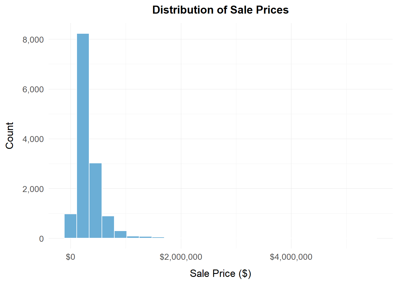
Distribution of Sales Prices - Histogram

The distribution of sales prices is heavily skewed right, with a high percentage of thee transactions below $500,000, and a relatively small number of homes falling in the multi-million dollar range. This chart also also gives insight into the potential presence of high leverage outliers falling toward the left. A concentration of thousands of sales clustered on the lower end of the price ranges suggests strong segmentation, meaning that the market is split into distinct groups, where you see a large cluster of homes that are relatively similar and a smaller but very different cluster of high-value properties with luxury features and few homes in-between, the market looks like separate groups rather than one gradually increasing scale. It’s important to note that this spread likely indicates heteroskedasticity, and would require a log transformation for statistical inference.

# Geographic distribution map - Sale Price

tmap_mode("plot")

sale_price_map <- tm_shape(philly_neighborhoods) +
  tm_polygons(col = "gray95", border.col = "gray65") +
  tm_shape(final_data) +
  tm_dots(col = "sale_price",
          palette = "YlOrRd",
          size = 0.05,
          style = "quantile",
          col.title = "Sale Price ($)") +
  tm_layout(main.title = "Geographic Distribution of Sale Prices",
            main.title.position = "center",
            main.title.size = 1.2,
            legend.outside = TRUE,
            frame = FALSE,
            bg.color = "#f5f4f0")

sale_price_map

#tmap_save(tm = sale_price_map, filename = "slide_images/geo-price-map.png", width = 10, height = 6, units = "in", dpi = 300, bg = "transparent")

Geographic Distribution of Sales Prices - Map

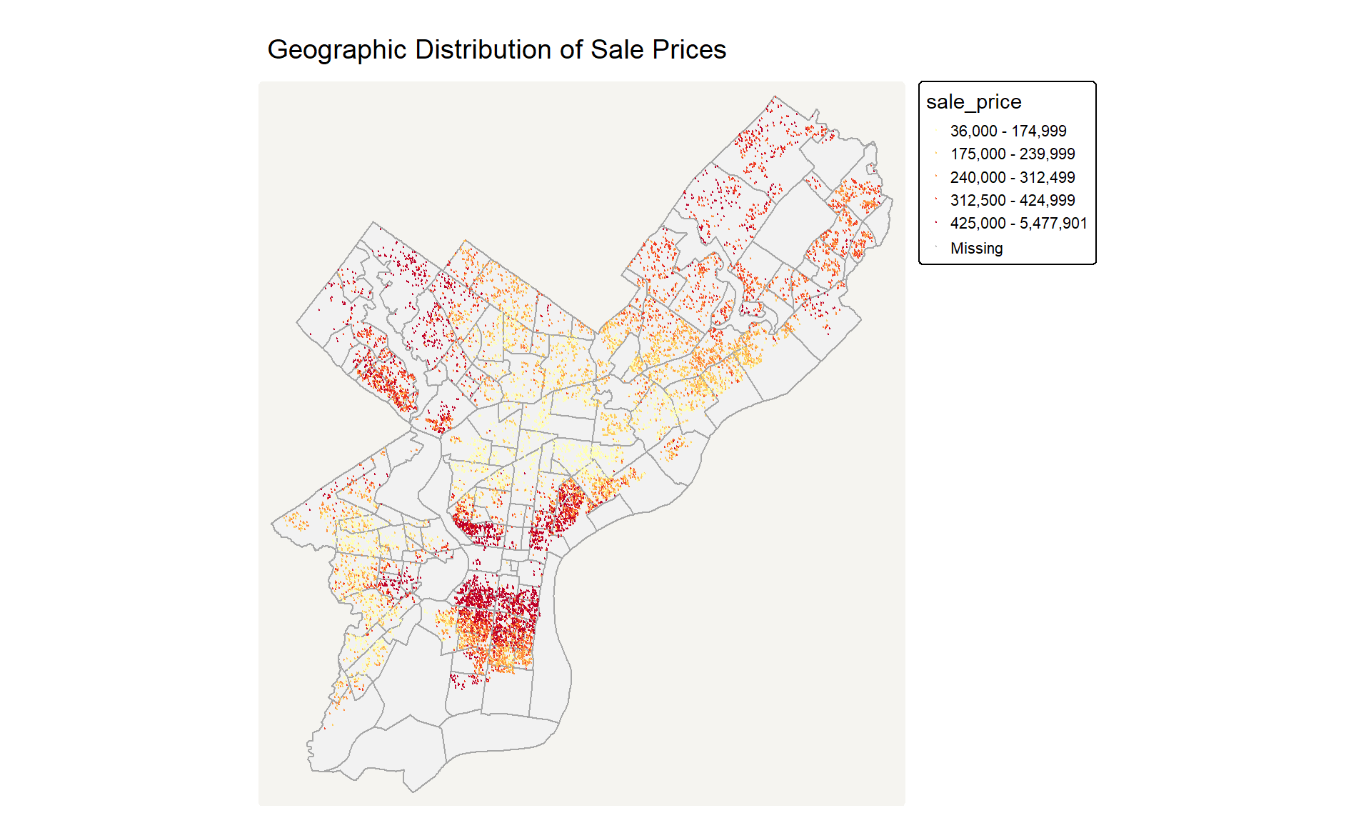
This map displays a high variation of sales prices distributed throughout the city. The higher priced clustered areas are the Center City, University City, the riverfront, and affluent pockets of the Northwest, potentially because these areas provide easy access to transit, employment centers, and cultural amenities. The northern area stretching above Broad Street into parts of West and North Philadelphia displays lower-priced homes, potentially reflecting long-term disinvestment, high vacancy rates, and aging non-renovated housing stock. The spatial clustering suggests that sale price is place-dependent in Philadelphia, mostly due to neighborhood qualities, and fixed effects.

# Sale Price vs structural features scatter plot

# Sale Price vs. Square feet 
price_v_sqft_plot <- ggplot(final_data, aes(x = square_feet, y = sale_price)) +
  geom_point(alpha = 0.4, color = "#08519C", size = 1.3) +
  geom_smooth(method = "lm", se = FALSE, color = "red", linewidth = 1) +
  labs(title = "Sale Price vs. Square Feet",
       x = "Square Feet",
       y = "Sale Price ($)") +
  scale_x_continuous(labels = scales::comma) +
  scale_y_continuous(labels = scales::dollar) +
  theme_minimal(base_size = 13) +
  theme(
    panel.background = element_rect(fill = "#f5f4f0"),
    panel.grid.major = element_line(color = "gray90", size = 0.3),
    panel.grid.minor = element_line(color = "gray95", size = 0.2),
    plot.title = element_text(hjust = 0.5, face = "bold", size = 14, margin = margin(b = 10)),
    axis.title.x = element_text(margin = margin(t = 10)),
    axis.title.y = element_text(margin = margin(r = 10))
    )

price_v_sqft_plot

#ggsave("slide_images/price-v-sqft.png", plot = price_v_sqft_plot, width = 6, height = 4, units = "in", dpi = 300)

Sale Price vs. Square Feet

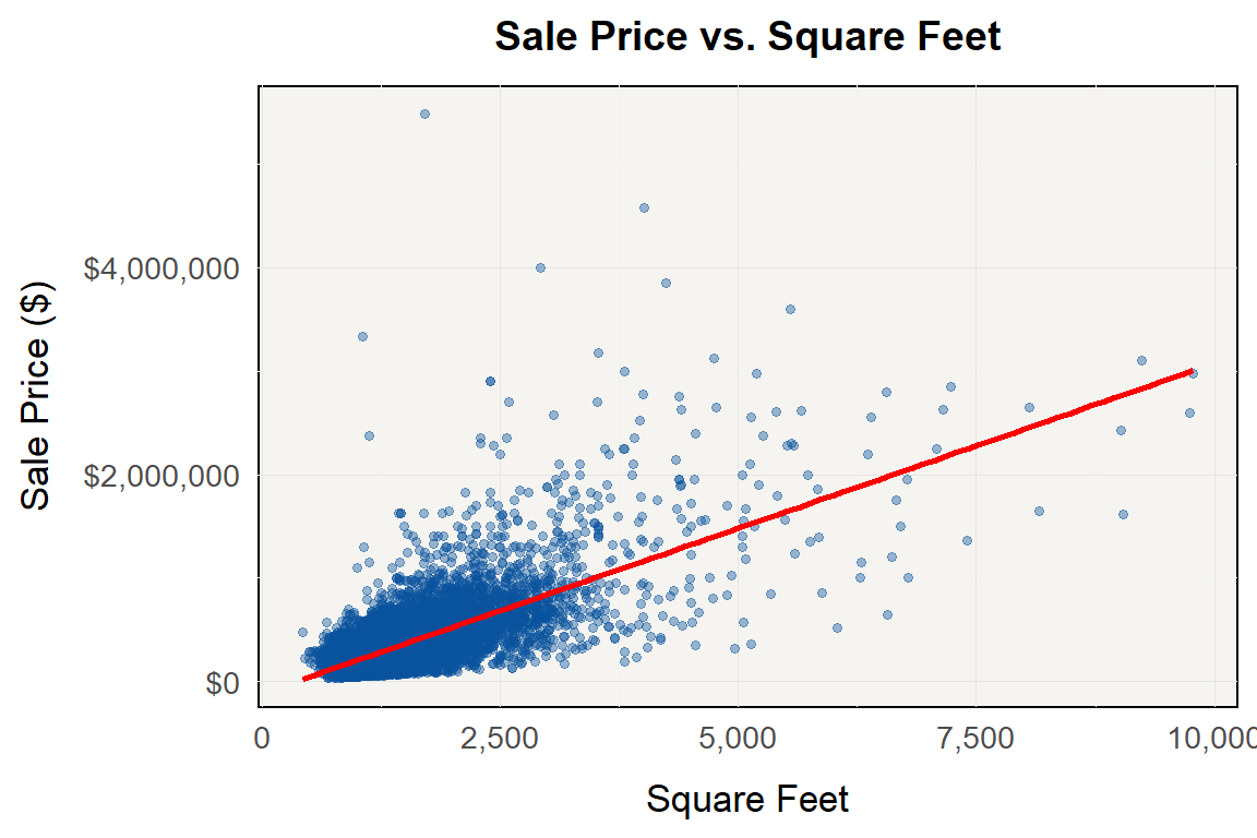
This scatter plot highlights the importance of home size as a structural indicator of value, even though the relationship may not be linear. There is a dense concentration of homes clustered below 3,000 sq ft. and under $500,000 consistent with the sales price distribution. Here we are seeing the same strong skew to the right, displaying a relationship between the two variables. The upward trend is fairly obvious, larger homes = an increase in price, however the spread gets wider as square footage increases, indicating that while square footage is positively associated with price, the weaker relationship among larger properties suggests that additional living space contributes less to value once the home reaches a certain size category.

# Sale Price vs. Number of Fireplaces 

price_v_fire_plot <- ggplot(final_data, aes(x = fireplace_num, y = sale_price)) +
  geom_jitter(alpha = 0.5, color = "#08519C", size = 1.3, width = 0.15, height = 0) +
  geom_smooth(method = "lm", se = FALSE, color = "red", linewidth = 1) +
  labs(title = "Sale Price vs. Number of Fireplaces",
       x = "Number of Fireplaces",
       y = "Sale Price ($)") +
  scale_x_continuous(labels = scales::comma) +
  scale_y_continuous(labels = scales::dollar) +
  theme_minimal(base_size = 13) +
  theme(
    panel.background = element_rect(fill = "#f5f4f0"),
    panel.grid.major = element_line(color = "gray90", size = 0.3),
    panel.grid.minor = element_line(color = "gray95", size = 0.2),
    plot.title = element_text(hjust = 0.5, face = "bold", size = 14, margin = margin(b = 10)),
    axis.title.x = element_text(margin = margin(t = 10)),
    axis.title.y = element_text(margin = margin(r = 10))
    )

price_v_fire_plot

#ggsave("slide_images/price-v-fire.png", plot = price_v_fire_plot, width = 6, height = 4, units = "in", dpi = 300)

Sale Price vs. Number of Fireplaces

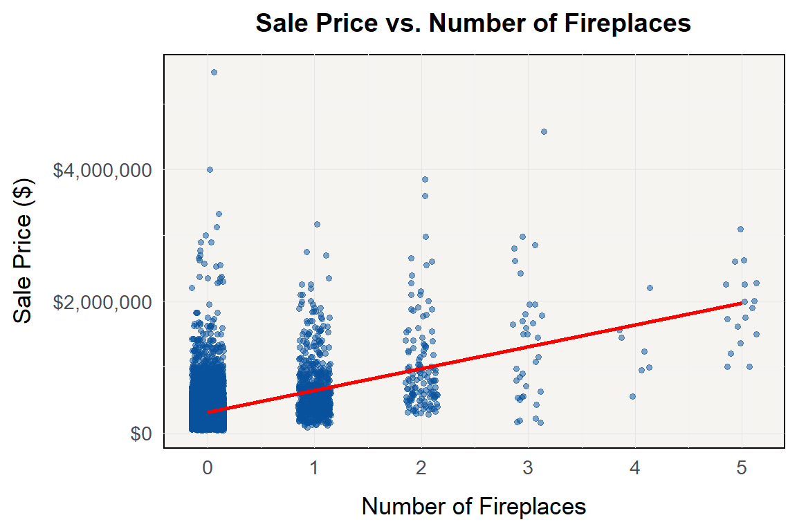
This chart displays the positive relationship between the value of a home in relation to the quality and character of aesthetic features. Nearly all homes with no fireplaces remain in the lower-mid price range, and once a home has two or more fire places the sale price increases to a much higher range. Homes in Philadelphia with several fireplaces are usually bigger, older, homes with higher-end finishes, meaning that fireplace count can serve as a secondary and indirect indicator of several other indicators that influence home value, and this is the reason for the high level of noise on the chart.

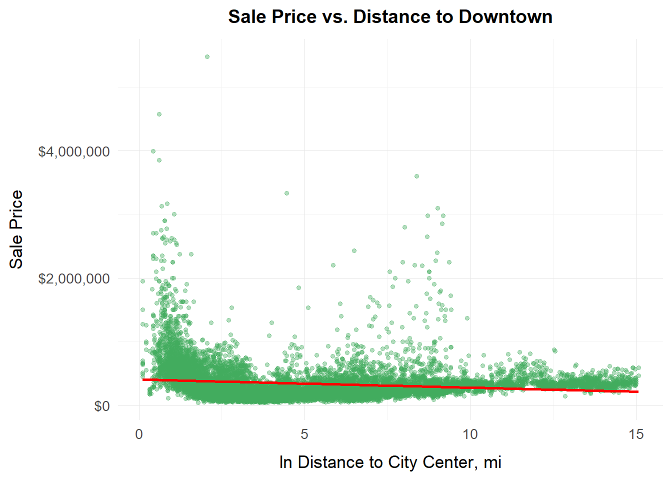
# Sale Price vs. Spatial Features

# Sale Price vs Distance to city center
price_v_spatial_plot <- ggplot(final_data, aes(x = city_dist_mi, y = sale_price)) +
  geom_point(alpha = 0.4, color = "#41AB5D", size = 1.3) +
  geom_smooth(method = "lm", se = FALSE, color = "red", linewidth = 1) +
  labs(title = "Sale Price vs. Distance to Downtown",
       x = "ln Distance to City Center, mi",
       y = "Sale Price") +
  scale_x_continuous(labels = scales::comma) +
  scale_y_continuous(labels = scales::dollar) +
  theme_minimal(base_size = 13) +
  theme(
    panel.grid.major = element_line(color = "gray90", size = 0.3),
    panel.grid.minor = element_line(color = "gray95", size = 0.2),
    plot.title = element_text(hjust = 0.5, face = "bold", size = 14, margin = margin(b = 10)),
    axis.title.x = element_text(margin = margin(t = 10)),
    axis.title.y = element_text(margin = margin(r = 10))
    )

price_v_spatial_plot

Sale Price vs. Distance to City Center

The plots shows a weak negative relationship between price and distance to the city center. High valued homes fall both close to downtown and well outside of it, highlighting the structure of Philadelphia’s housing market as it relates to location. It’s not a city where closer is always better, instead certain neighborhoods like chestnut hill maintain their high premiums due to neighborhood reputation, and school quality. This pattern suggests that there are many fixed affects at play here, and it is important to note that similar patterns were displayed among many spatial variables.

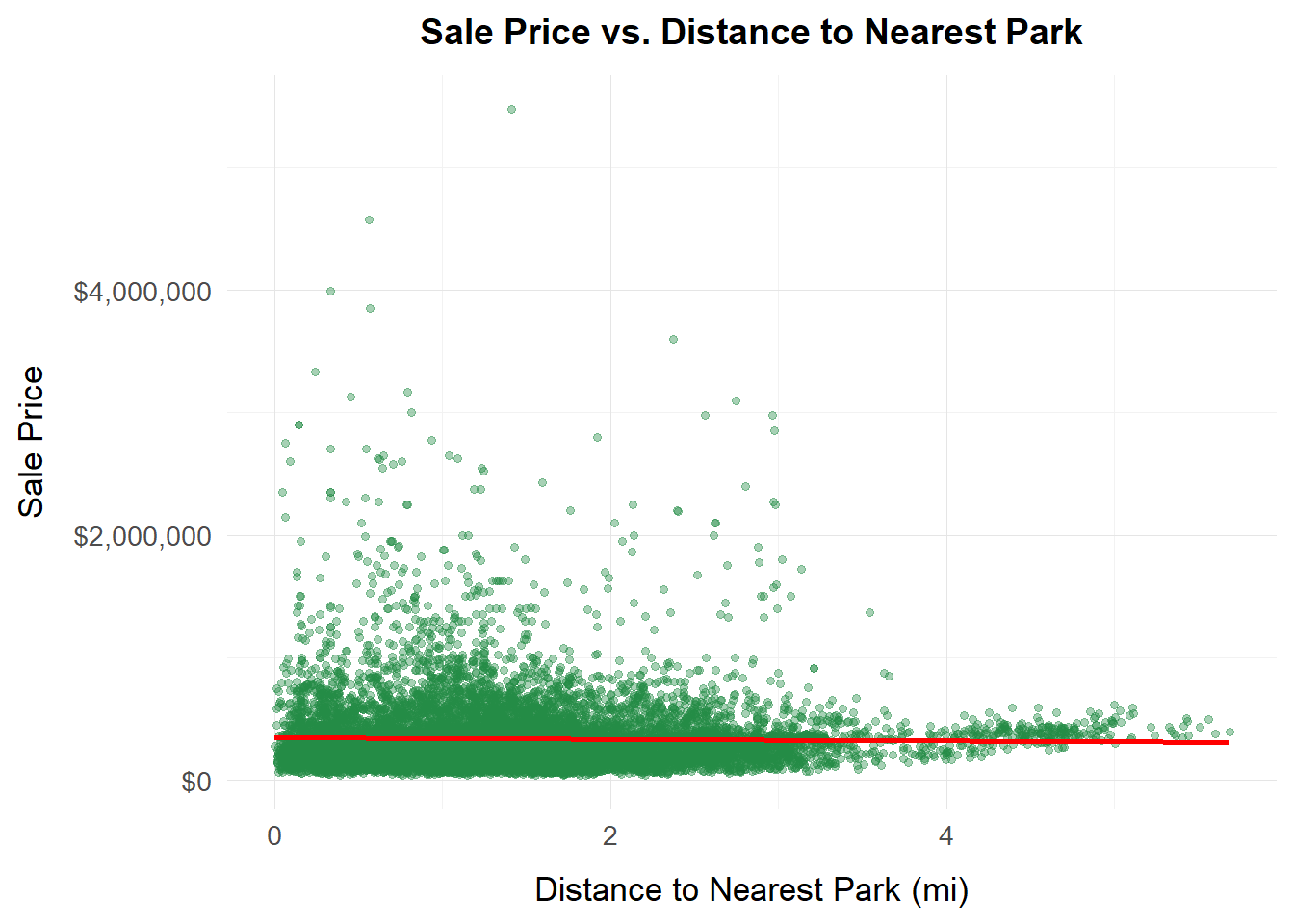
# Sale Price vs. Distance to Parks - Park Accessibility

price_v_park_plot <- ggplot(final_data, aes(x = parks_mile, y = sale_price)) +
  geom_point(alpha = 0.4, color = "#238B45", size = 1.3) +
  geom_smooth(method = "lm", se = FALSE, color = "red", linewidth = 1) +
  labs(title = "Sale Price vs. Distance to Nearest Park",
       x = "Distance to Nearest Park (mi)",
       y = "Sale Price") +
  scale_x_continuous(labels = scales::comma) +
  scale_y_continuous(labels = scales::dollar) +
  theme_minimal(base_size = 13) +
  theme(
    panel.grid.major = element_line(color = "gray90", size = 0.3),
    panel.grid.minor = element_line(color = "gray95", size = 0.2),
    plot.title = element_text(hjust = 0.5, face = "bold", size = 14, margin = margin(b = 10)),
    axis.title.x = element_text(margin = margin(t = 10)),
    axis.title.y = element_text(margin = margin(r = 10))
    )

price_v_park_plot

Sale Price vs. Distance to Parks - Park Accessibility

The plot suggests that distance to parks has very little trend with sale price. Many high-priced properties sit both very close and very far away from parks, suggesting that park accessibility alone may not hold much value. This could be correlated with the fact that some parks are major attractions; i.e Fairmount Park, while others have limited impact on neighborhood desirability, especially in areas of low investment. Because of the difference in park quality across the city, the distance metric may not represents the true relationship, and more neighborhood or amenity variables may be required to capture environmental quality more accurately.

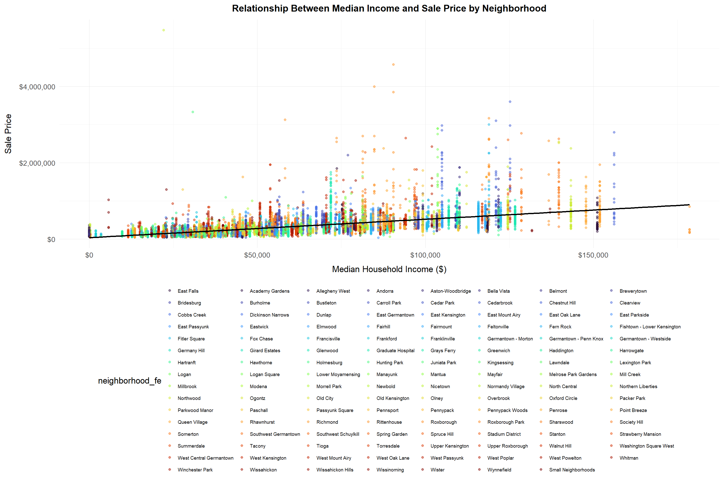
# Median income vs Sale Price per neighborhood

inc_v_price_plot <- ggplot(final_data, aes(x = medhhinc, y = sale_price, color = neighborhood_fe)) +
  geom_point(alpha = 0.5) +
  geom_smooth(method = "lm", se = FALSE, color = "black") +
  labs(title = "Relationship Between Median Income and Sale Price by Neighborhood",
       x = "Median Household Income ($)",
       y = "Sale Price") +
  scale_x_continuous(labels = scales::dollar) +
  scale_y_continuous(labels = scales::dollar) +
  scale_color_viridis_d(option = "turbo") +
  theme_minimal(base_size = 13) +
  theme(
    panel.grid.major = element_line(color = "gray90", size = 0.3),
    panel.grid.minor = element_line(color = "gray95", size = 0.2),
    plot.title = element_text(hjust = 0.5, face = "bold", size = 14, margin = margin(b = 10)),
    axis.title.x = element_text(margin = margin(t = 10)),
    axis.title.y = element_text(margin = margin(r = 10)),
    legend.position = "bottom",
    legend.text = element_text(size = 7),
    legend.key.size = unit(0.4, "cm"),
    legend.box = "horizontal"
    ) +
  guides(color = guide_legend(ncol = 8, byrow = TRUE))

inc_v_price_plot

Median Income vs Sale Price per neighborhood

This plot further advances the claim that even with a lot of scatter in the points, there is a noticeable upward trend of homes in higher-income neighborhoods selling for higher prices. Many of the neighborhoods cluster in specific ranges of the price scale, even when income levels are similar, suggesting that the housing market in Philadelphia is dependent not only on demographics or income, but place effects, where reputation or fixed effects in a neighborhood increase or reduce prices. An example of this is some neighborhoods with moderate household incomes still show clusters of high-value transactions, while others with similar incomes remain in the lower end of the market, again highlighting other factors and fixed effects like transit access, historical character, and school quality. The main takeaway is that while higher-income neighborhood tend to have homes with higher sale prices, neighborhood identity also plays a big role in sale price.

# Spatial Relationship Between sale price and structural predictors

tmap_mode("plot")

# Sale Price
map_value <- tm_shape(philly_tracts[philly_tracts$COUNTYFP == 101, ]) +
  tm_polygons(col = "gray90", border.col = "gray45", lwd = 0.5) +
  tm_shape(final_data) +
  tm_dots(col = "sale_price",
          palette = "YlOrRd",
          style = "quantile",
          size = 0.04,
          title = "Sale Price") +
  tm_layout(main.title = "Distribution of Sale Prices",
            main.title.position = "center",
            main.title.size = 1.2,
            legend.outside = TRUE,
            frame = FALSE)

# Bathrooms Predictor

map_bath <-  tm_shape(philly_tracts[philly_tracts$COUNTYFP == 101, ]) +
  tm_polygons(col = "gray90", border.col = "gray45", lwd = 0.5) +
  tm_shape(final_data) +
  tm_dots(col = "bath_num",
          palette = "Blues",
          style = "quantile",
          size = 0.04,
          title = "Number of Bathrooms") +
  tm_layout(main.title = "Distribution of Bathrooms",
            main.title.position = "center",
            main.title.size = 1.2,
            legend.outside = TRUE,
            frame = FALSE)

# Stories Predictor

map_story <-  tm_shape(philly_tracts[philly_tracts$COUNTYFP == 101, ]) +
  tm_polygons(col = "gray90", border.col = "gray45", lwd = 0.5) +
  tm_shape(final_data) +
  tm_dots(col = "story_num",
          palette = "Greens",
          style = "quantile",
          size = 0.04,
          title = "Number of Stories") +
  tm_layout(main.title = "Distribution of Stories",
            main.title.position = "center",
            main.title.size = 1.2,
            legend.outside = TRUE,
            frame = FALSE)

# Display them side by side

tmap_arrange(map_value, map_bath, map_story, ncol = 3)

map_struct <- tmap_arrange(map_value, map_bath, map_story, ncol = 3)

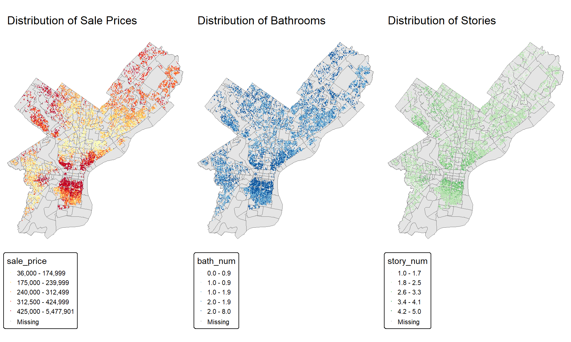
Spatial Relationship Between sale price and structural predictors (bathrooms and stories) - Map

This figure shows how housing characteristics are clustered across Philadelphia. Here we can see the sale price distribution directly against certain structural features. Bathrooms and number of stories follow similar geographic patterns, as sale price, areas with higher sales prices tend to have bigger homes with more bathrooms and more stories. In contrast, neighborhoods where homes have less structural amenities also have subsequently lower sale prices. This group of maps makes a strong visual argument that structural features and neighborhood context evolve together, supporting the modeling strategy of incorporating more structural than spatial predictors.

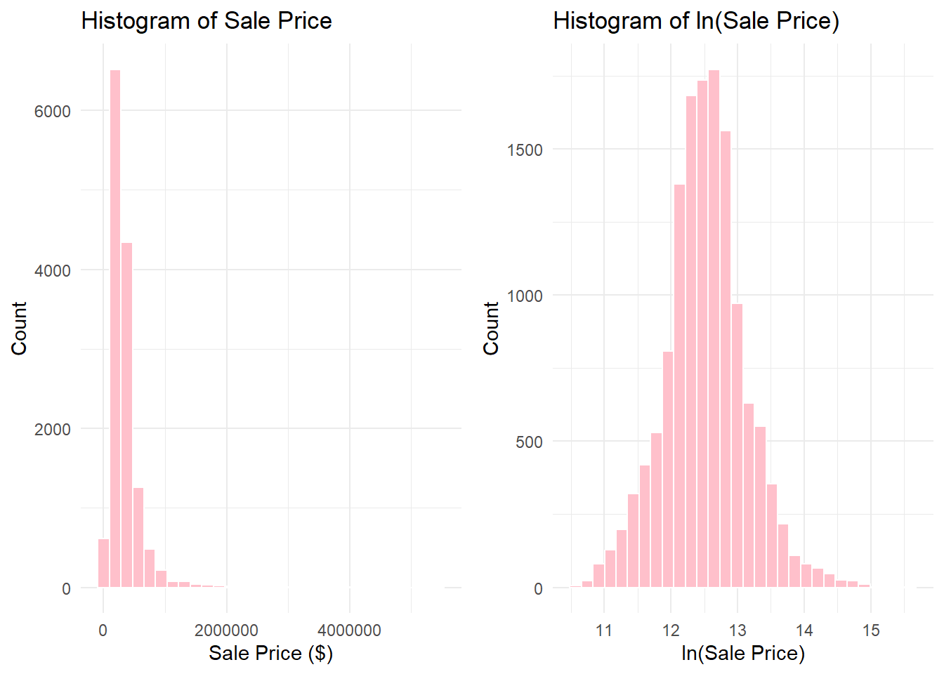
# Sale price histogram.
price_hist <- ggplot(residential_points, aes(x = sale_price)) +
  geom_histogram(fill = "pink", color = "white") +
  labs(title = "Histogram of Sale Price", x = "Sale Price ($)", y = "Count") +
  theme_minimal()

# Log sale price histogram.
ln_price_hist <- ggplot(residential_points, aes(x = ln_sale_price)) +
  geom_histogram(fill = "pink", color = "white") +
  labs(title = "Histogram of ln(Sale Price)", x = "ln(Sale Price)", y = "Count") +
  theme_minimal()

grid.arrange(price_hist, ln_price_hist, ncol = 2)

The raw distribution of sale prices is right-skewed with a median of 250,000 USD and a mean of 343,867 USD. There is a substantial gap in price between the third quartile (375,000 USD) and the maximum price (15,428,633 USD). While 75% of houses sold for 375,000 USD or less, the upper 25% exhibits considerable variability, with prices ranging up to 15.4 million USD, affecting the tail distribution. This suggests that a small number of luxury properties are affecting the distribution of the sales price data To address this skewness and improve model performance, we performed a log transformation, making our data closer to normal by compressing the scale of higher values, emphasizing a standardized change in percentage over dollar amount.

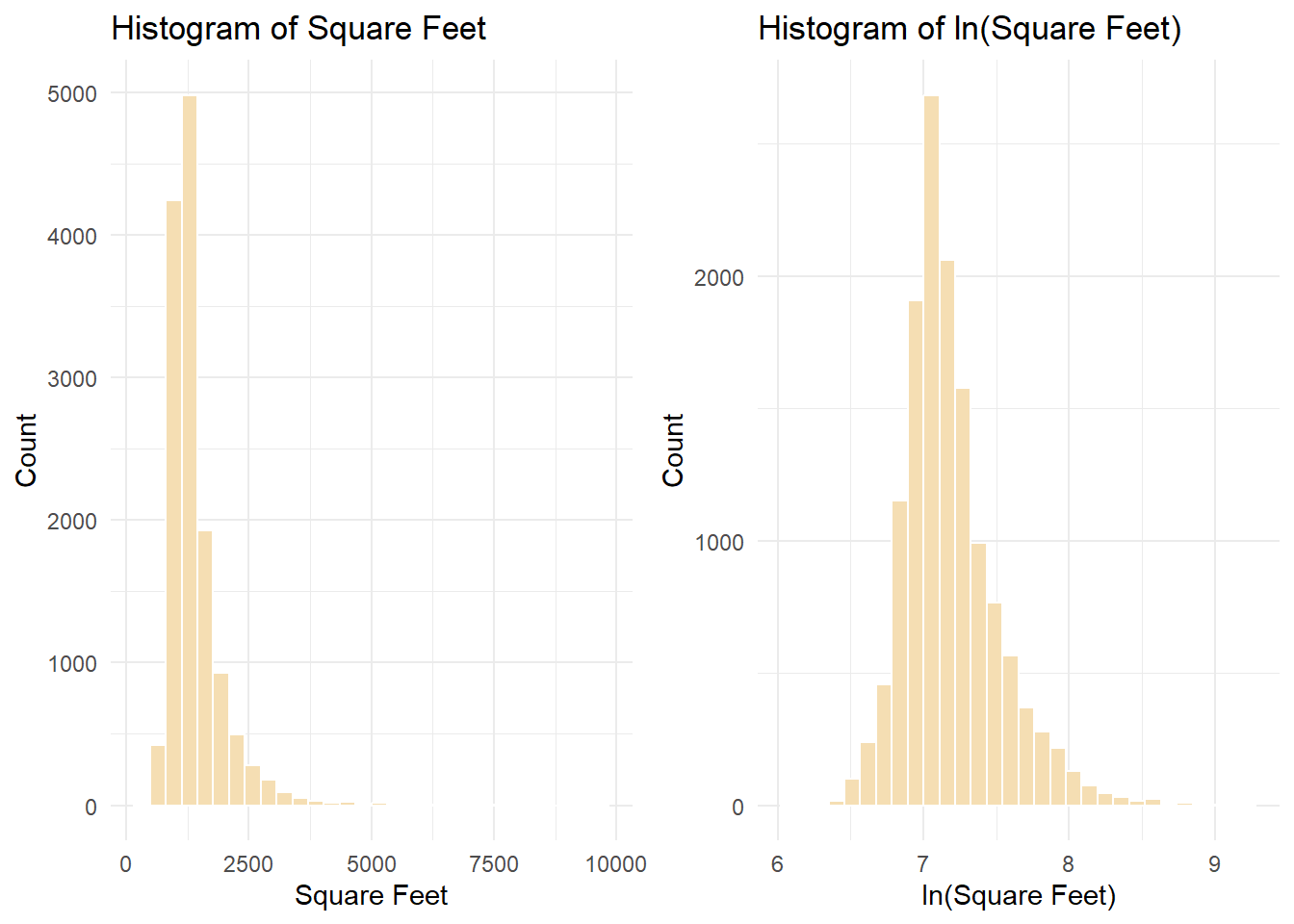
# Livable space histogram.
livable_area_hist <- ggplot(residential_points, aes(x = square_feet)) +
  geom_histogram(fill = "wheat", color = "white") +
  labs(title = "Histogram of Square Feet", x = "Square Feet", y = "Count") +
  theme_minimal()

# Log livable space histogram.
ln_square_feet_hist <- ggplot(residential_points, aes(x = ln_square_feet)) +
  geom_histogram(fill = "wheat", color = "white") +
  labs(title = "Histogram of ln(Square Feet)", x = "ln(Square Feet)", y = "Count") +
  theme_minimal()

grid.arrange(livable_area_hist, ln_square_feet_hist, ncol = 2)

The distribution of livable area is right-skewed, with a median of 1,216 sq ft and a mean of 1,372 sq ft. While 75% of homes are under 1,509 sq ft, a small number of larger properties extend the upper tail of the distribution. Notably, homes above 3,000 sq ft become increasingly sparse, suggesting a separation between standard and luxury housing markets. We applied a log transformation to this variable to create a more symmetric distribution by compressing the scale of larger homes, which improves linearity in our model and allows coefficients to represent proportional rather than absolute changes in square footage.

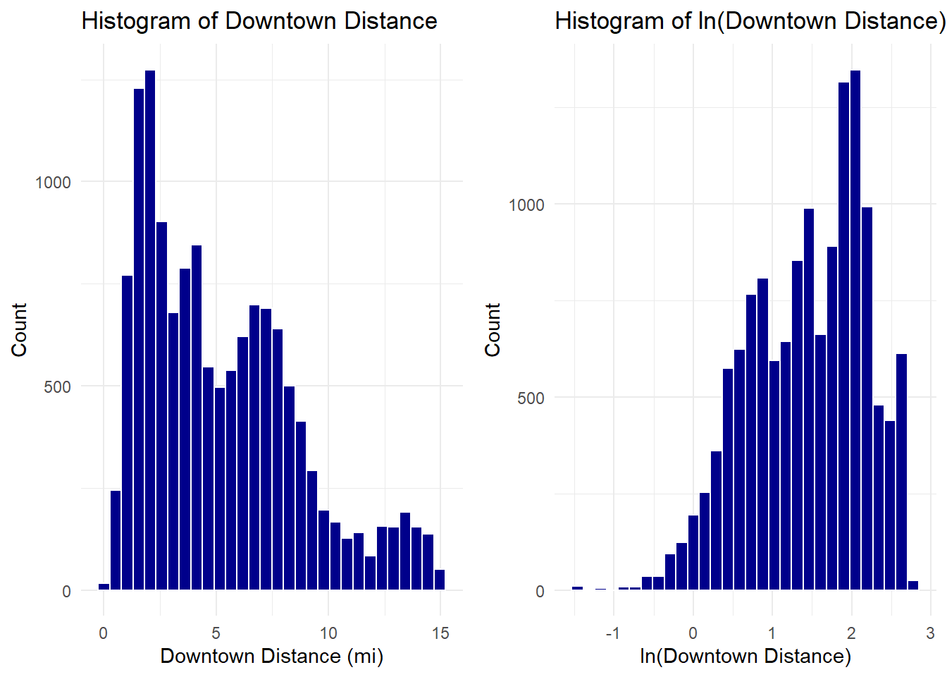
# Distance to downtown histogram.
downtown_dist_hist <- ggplot(residential_points, aes(x = city_dist_mi)) +
  geom_histogram(fill = "darkblue", color = "white") +
  labs(title = "Histogram of Downtown Distance", x = "Downtown Distance (mi)", y = "Count") +
  theme_minimal()

# Log distance to downtown histogram.
ln_downtown_dist_hist <- ggplot(residential_points, aes(x = ln_city_dist)) +
  geom_histogram(fill = "darkblue", color = "white") +
  labs(title = "Histogram of ln(Downtown Distance)", x = "ln(Downtown Distance)", y = "Count") +
  theme_minimal()

grid.arrange(downtown_dist_hist, ln_downtown_dist_hist, ncol = 2)

The distribution of distance to Center City (City Hall) is right-skewed, with fewer observations of houses occurring as the distance from Center City/City Hall increases. The effect of distance on housing prices is non-linear: being 1 mile from Center City has a larger impact on price than being 6 vs. 11 miles out. To account for this, we applied a log transformation, which compresses the upper tail, creates a more symmetric distribution, and reduces the influence of extreme distances. This transformation improves linearity in our regression model and allows coefficients to be interpreted as proportional changes in price per proportional change in distance.

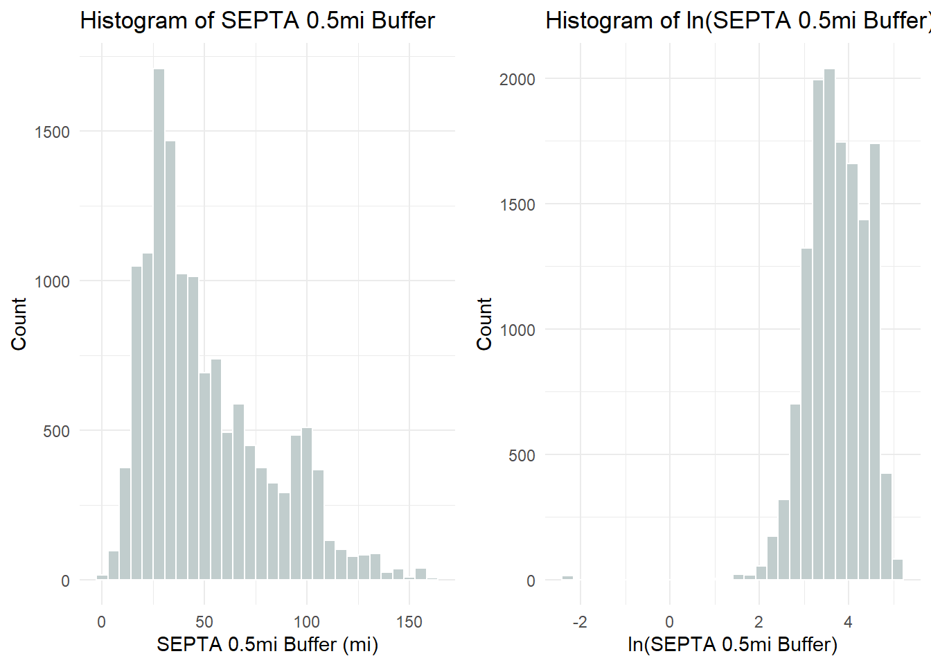
# SEPTA buffer histogram.
septa_buffer_hist <- ggplot(residential_points, aes(x = septa_half_mi)) +
  geom_histogram(fill = "azure3", color = "white") +
  labs(title = "Histogram of SEPTA 0.5mi Buffer", x = "SEPTA 0.5mi Buffer (mi)", y = "Count") +
  theme_minimal()

# Log SEPTA buffer histogram.
ln_septa_buffer_hist <- ggplot(residential_points, aes(x = ln_septa_half_mi)) +
  geom_histogram(fill = "azure3", color = "white") +
  labs(title = "Histogram of ln(SEPTA 0.5mi Buffer)", x = "ln(SEPTA 0.5mi Buffer)", y = "Count") +
  theme_minimal()

grid.arrange(septa_buffer_hist, ln_septa_buffer_hist, ncol = 2)

The distribution of SEPTA access within a 0.5-mile buffer of each property is right-skewed, with a median of 44 and a mean of 52.5. While most properties have between 29 and 69 nearby SEPTA access points, there is substantial variation ranging from zero (likely remote suburban properties) to over 160 in the most transit-dense neighborhoods. The log transformation compresses this wide range and produces a more symmetric distribution, which is appropriate given that transit accessibility exhibits diminishing returns—the marginal benefit of additional access decreases as the total number increases.

# kNN amenities histogram.
knn_amenities_hist <- ggplot(residential_points, aes(x = knn_amenity_mi)) +
  geom_histogram(fill = "darkseagreen", color = "white") +
  labs(title = "Histogram of kNN Amenities", x = "kNN Amenities (mi)", y = "Count") +
  theme_minimal()

grid.arrange(knn_amenities_hist)

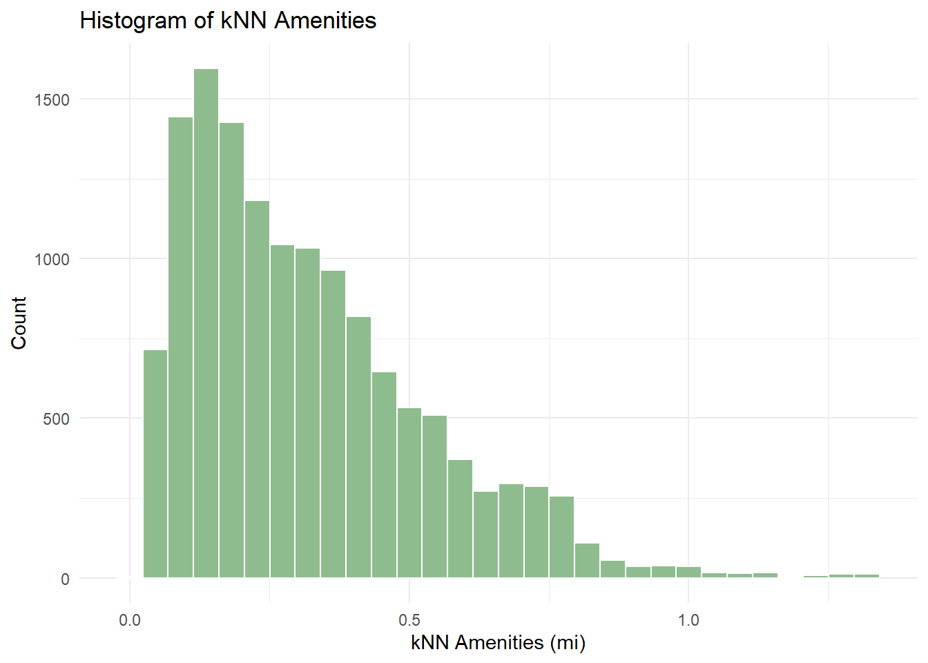
For the kNN Amenities variable, the mean distance to the nearest amenity per household is 0.31 miles, and the median is 0.27 miles. Seventy-five percent of households are within 0.42 miles of any of the 23 amenities described in the data cleaning section. These statistics showcase Philadelphia’s reputation as a highly walkable city. Observations beyond 1 mile typically reflect suburban or rural settings. We did not transform this variable, instead using the raw distances to preserve the direct relationship between amenity proximity and property values.The kNN approach inherently reflects local amenity density, with shorter distances in denser areas and longer distances where households are more dispersed.

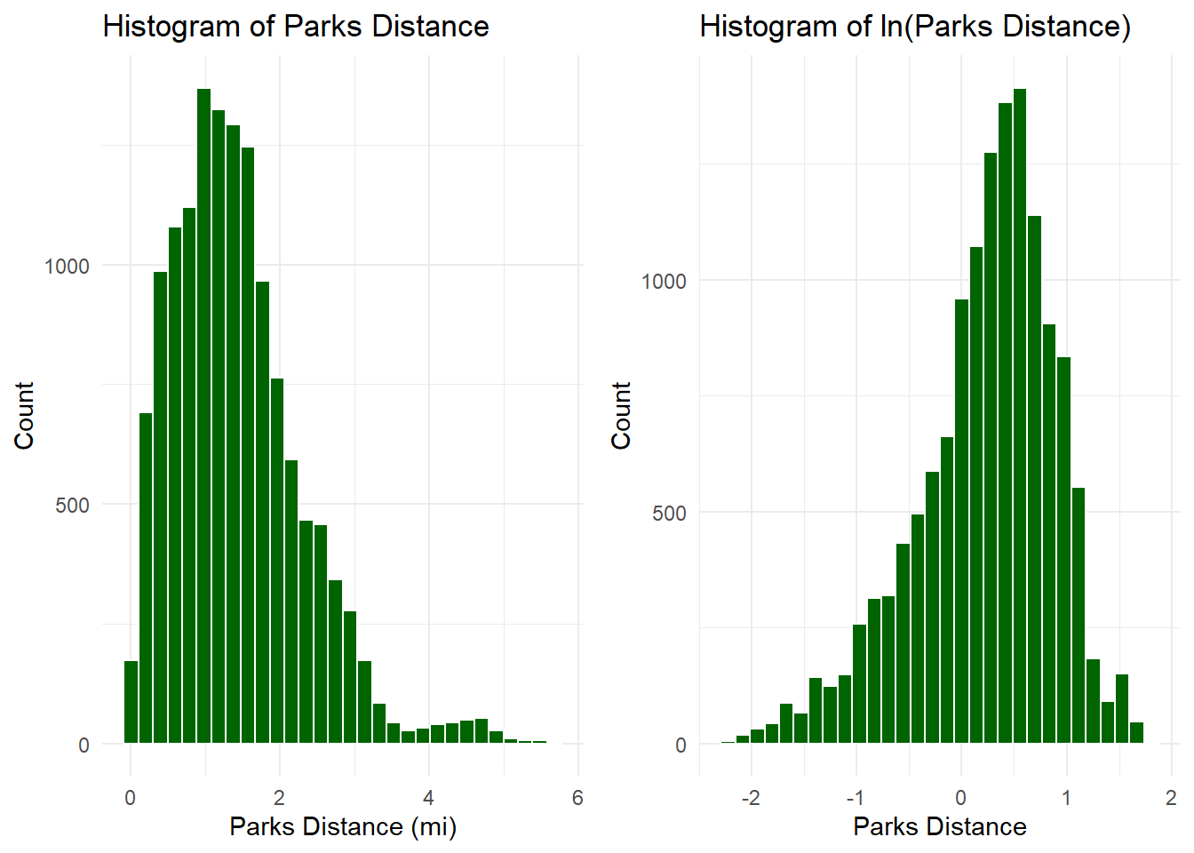
# Distance to park histogram..
parks_dist <- ggplot(residential_points, aes(x = parks_mile)) +
  geom_histogram(fill = "darkgreen", color = "white") +
  labs(title = "Histogram of Parks Distance", x = "Parks Distance (mi)", y = "Count") +
  theme_minimal()

# Log distance to park histogram.
ln_parks_dist <- ggplot(residential_points, aes(x = ln_park_dist)) +
  geom_histogram(fill = "darkgreen", color = "white") +
  labs(title = "Histogram of ln(Parks Distance)", x = "Parks Distance", y = "Count") +
  theme_minimal()

grid.arrange(parks_dist, ln_parks_dist, ncol = 2)

The distribution of the variable Distance from Parks by miles is showing a slight right skew. Between the third quartile and the maximum there is a jump of about 3 miles, indicating outliers beyond 2 miles. Due to this, we chose to log the variable to ensure it is normal for our model.

# Number of bathrooms histogram.
ggplot(residential_points, aes(x = bath_num)) +
  geom_histogram(fill = "gold", color = "white") +
  labs(title = "Histogram of Bathrooms", x = "Bathrooms", y = "Count") +
  theme_minimal()

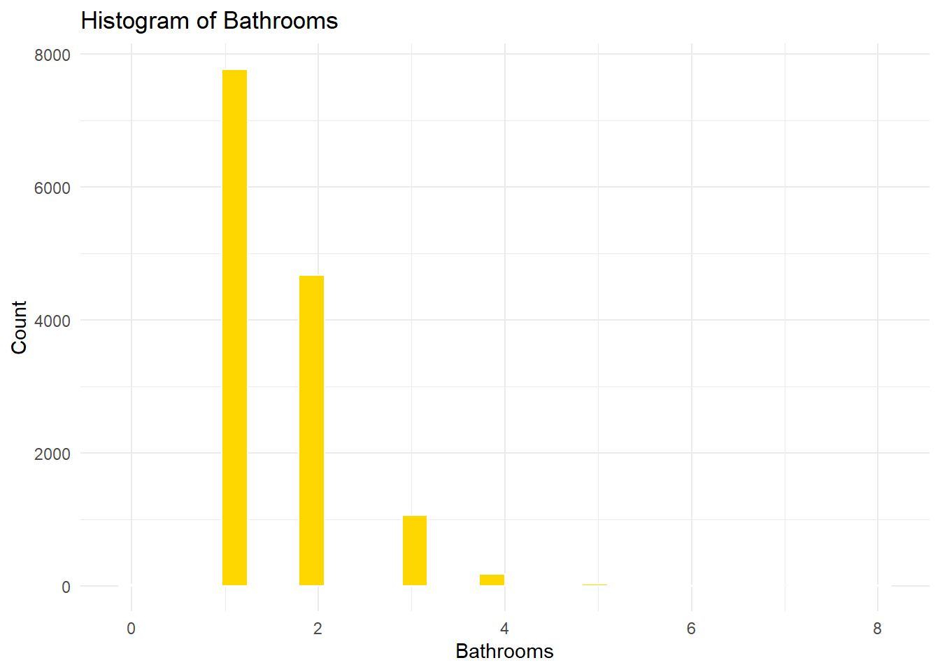
The histogram showcases the number of observations of properties with n bathrooms. Most observations exhibit 1 or 2 bathrooms per property, with a an outlier of 8 bathrooms.

# Number of fireplaces histogram.
ggplot(residential_points, aes(x = fireplace_num)) +
  geom_histogram(fill = "darkred", color = "white") +
  labs(title = "Histogram of Fireplaces", x = "Fireplaces", y = "Count") +
  theme_minimal()

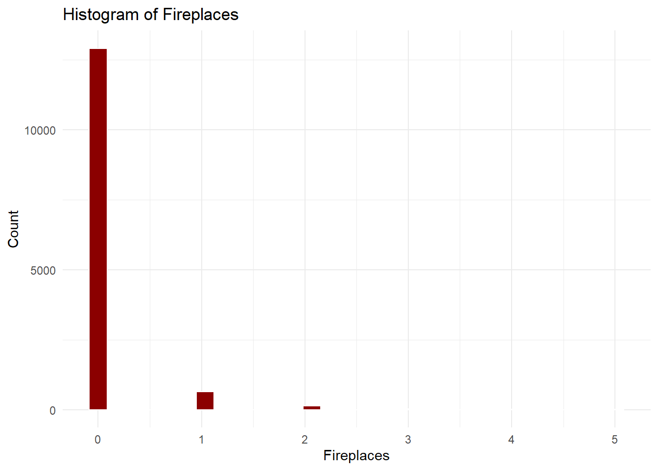
This histogram showcases the number of observations with n fireplaces. Most observations contain 0 fireplaces, with outliers of property(ies) containing 2 or more.

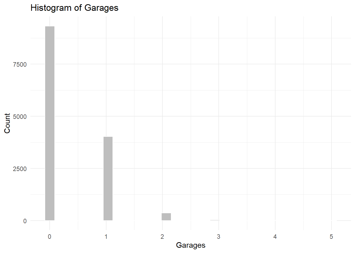
# Number of garages histogram.
ggplot(residential_points, aes(x = garage_num)) +
  geom_histogram(fill = "gray", color = "white") +
  labs(title = "Histogram of Garages", x = "Garages", y = "Count") +
  theme_minimal()

This histogram showcases the number of garages available per observation. The median is 0 garages per property, with a maximum of 5 garages per property.

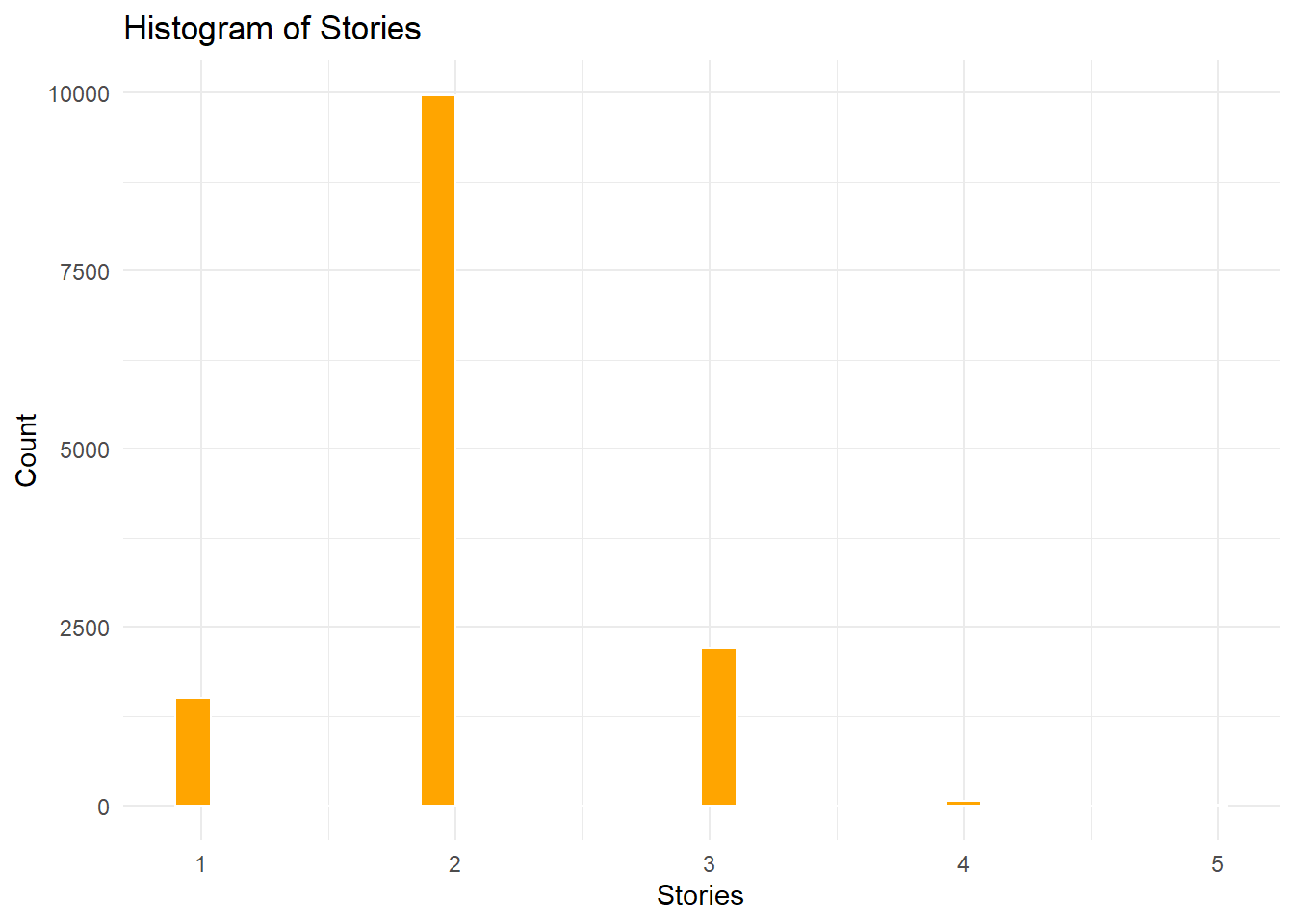
# Number of stories histogram.
ggplot(residential_points, aes(x = story_num)) +
  geom_histogram(fill = "orange", color = "white") +
  labs(title = "Histogram of Stories", x = "Stories", y = "Count") +
  theme_minimal()

This histogram showcases the number of observations that contain n housing stories. The median is 2 stories per property, with a maximum of 5 stories.

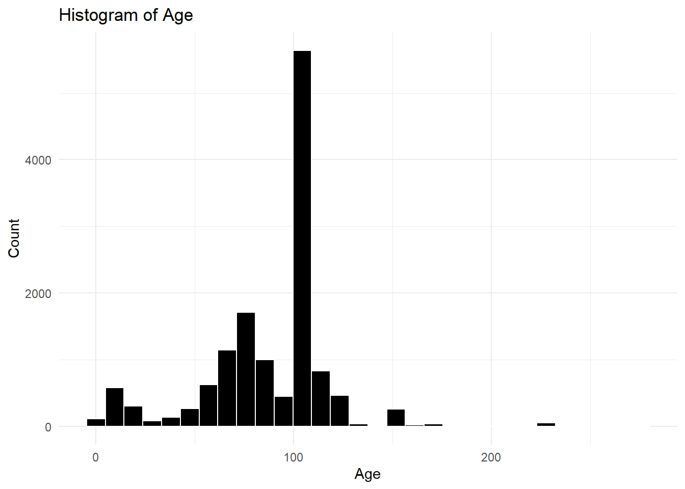
# Age histogram.
ggplot(residential_points, aes(x = age)) +
  geom_histogram(fill = "black", color = "white") +
  labs(title = "Histogram of Age", x = "Age", y = "Count") +
  theme_minimal()

This histogram showcases the amount of observations with their calculated ages (years) based off year built. The median age is 100 years, and the maximum is 275 years. This was then transformed into a polynomial variable to account for the decrease in housing price as the home ages until a certain age, then the price rises again.

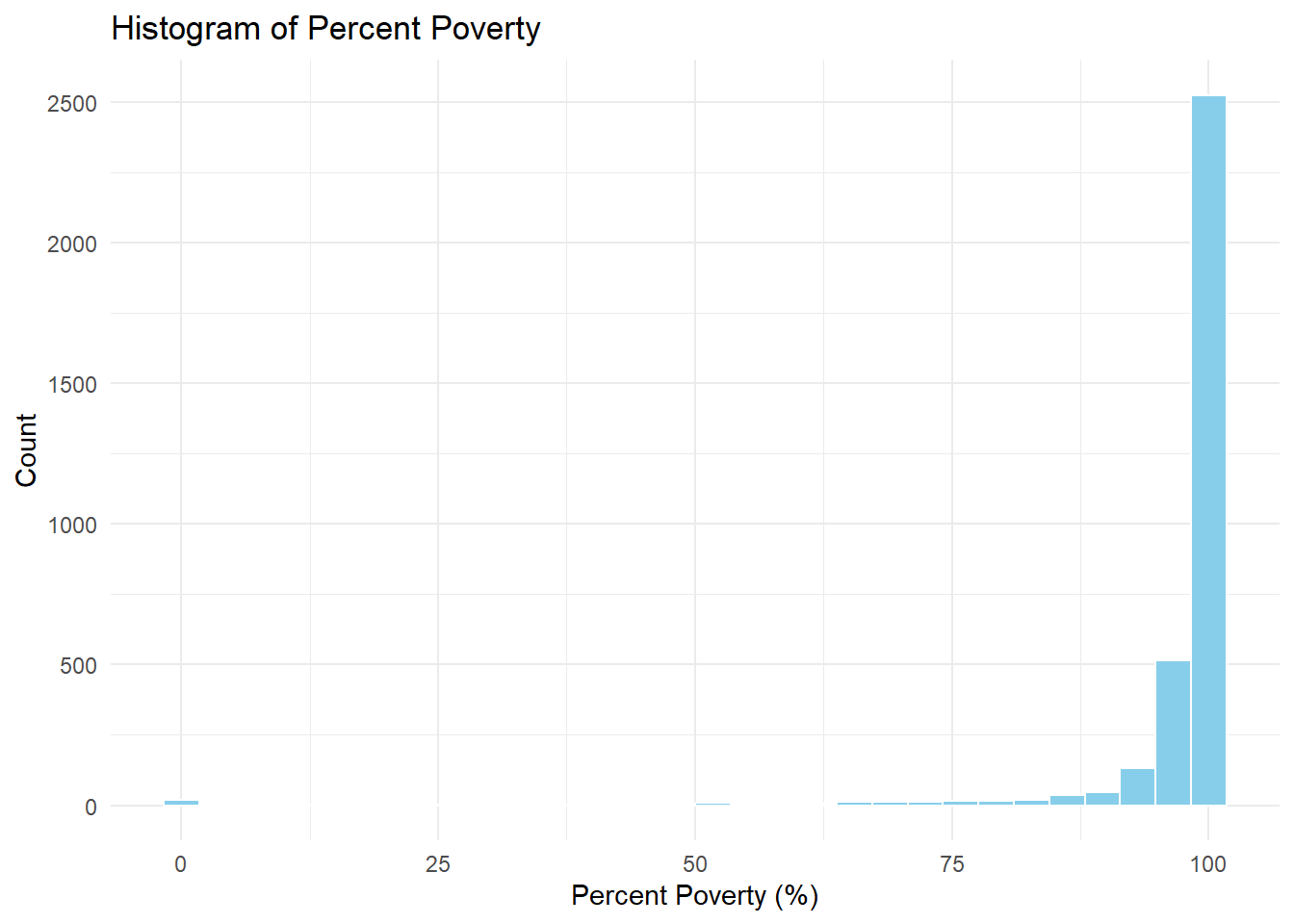
# Histogram for pct_poverty
ggplot(philly_acs_summary, aes(x = pct_poverty)) +
  geom_histogram(fill = "skyblue", color = "white") +
  labs(title = "Histogram of Percent Poverty", x = "Percent Poverty (%)", y = "Count") +
  theme_minimal()

This histogram presents the tracts with their determined percent poverty. The percentage is suspiciously high with the range from the minimum (0%) from the first quartile is 98 percent.We also have 32 tracts with no data.

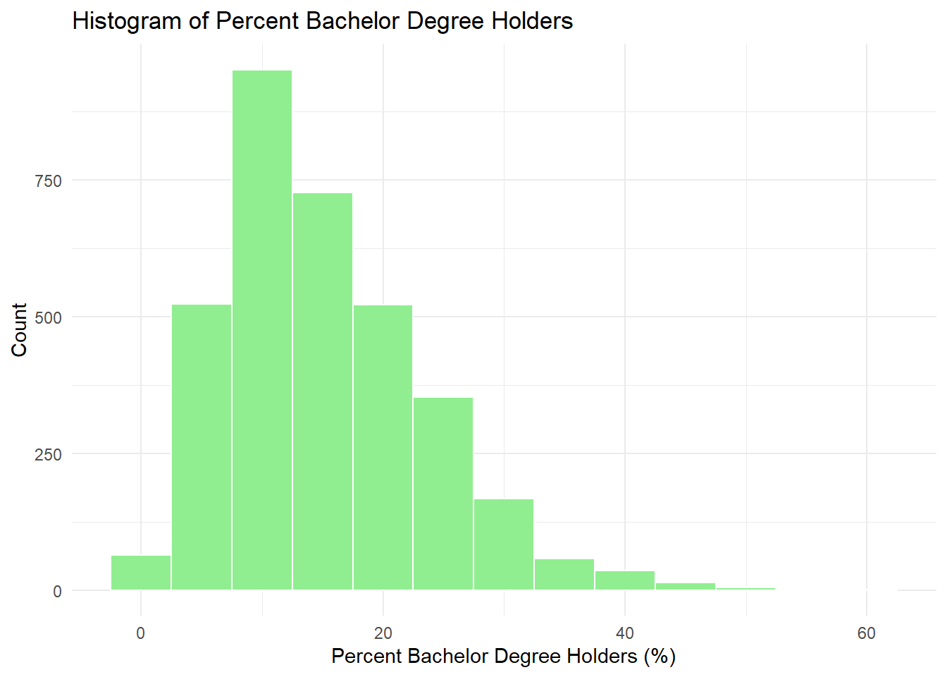
# Histogram for pct_bach
ggplot(philly_acs_summary, aes(x = pct_bach)) +
  geom_histogram(binwidth = 5, fill = "lightgreen", color = "white") +
  labs(title = "Histogram of Percent Bachelor Degree Holders", x = "Percent Bachelor Degree Holders (%)", y = "Count") +
  theme_minimal()

This histogram shows the distribution of percent of bachelor + degree holders per census tract. The median is 13.5 %, with most tracts falling between the minimum and third quartile. We also have 32 tracts with no data.

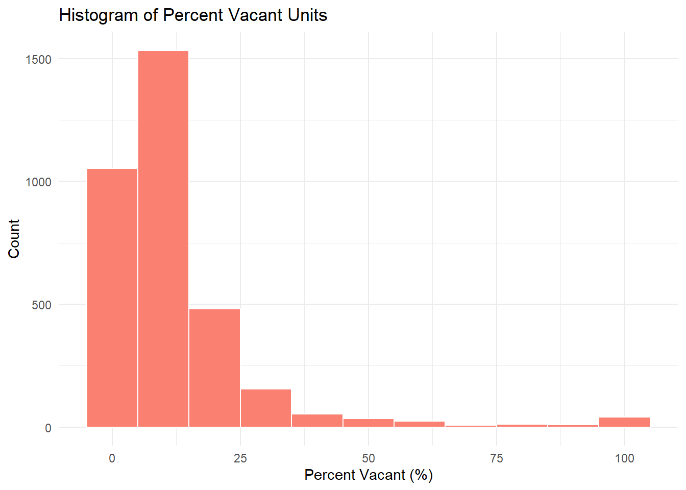
# Histogram for pct_vacant
ggplot(philly_acs_summary, aes(x = pct_vacant)) +
  geom_histogram(binwidth = 10, fill = "salmon", color = "white") +
  labs(title = "Histogram of Percent Vacant Units", x = "Percent Vacant (%)", y = "Count") +
  theme_minimal()

This histogram shows the distribution of percent vacant residences within the census tracts. The median percentage of vacant homes is 8 percent. We also have 44 tracts with no data.

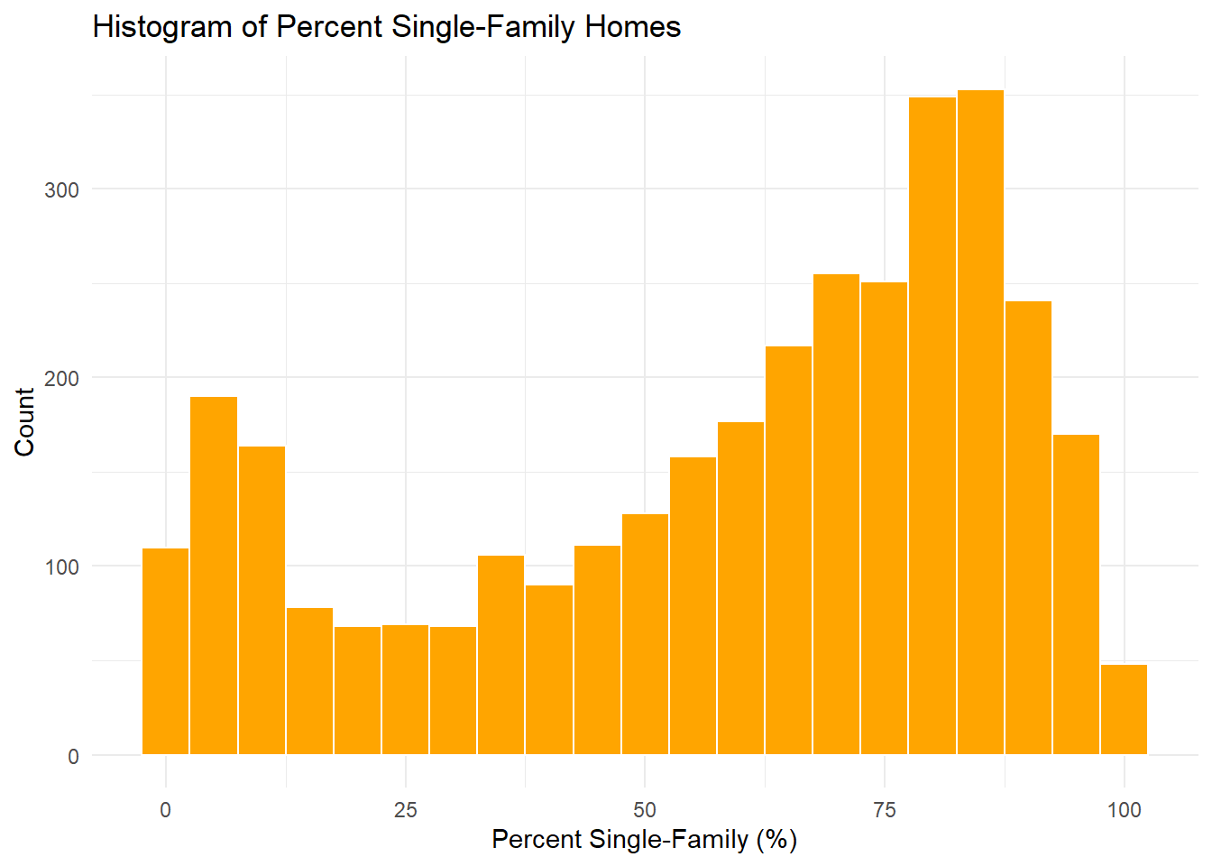
# Histogram for pct_single_family
ggplot(philly_acs_summary, aes(x = pct_single_family)) +
  geom_histogram(binwidth = 5, fill = "orange", color = "white") +
  labs(title = "Histogram of Percent Single-Family Homes ", x = "Percent Single-Family (%)", y = "Count") +
  theme_minimal()

This histogram represents the percent of single families per tract. The median for percent single families per tract is 66.58%. We also have 45 tracts with no data.

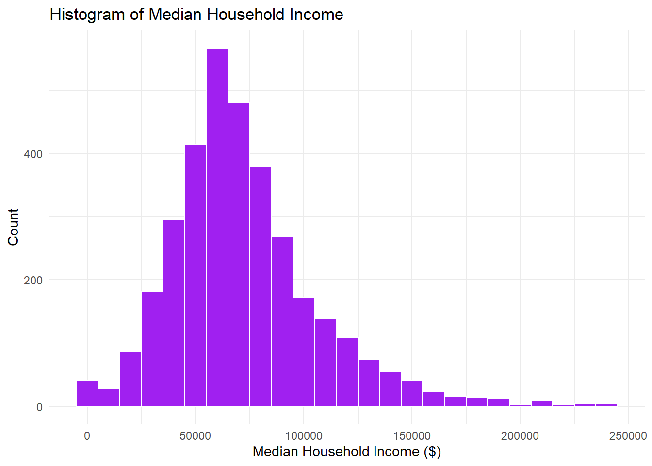
# Histogram for medhhinc
ggplot(philly_acs_summary, aes(x = medhhinc)) +
  geom_histogram(binwidth = 10000, fill = "purple", color = "white") +
  labs(title = "Histogram of Median Household Income", x = "Median Household Income ($)", y = "Count") +
  theme_minimal()

This histogram represents the median household income value per census tract. The median of the median household income value is $66,795. Slightly right-skewed. We also have 32 tracts with no data.

# Residential property correlation.
corr_matrix_df <- final_data %>%
  select(1:22) %>%
  st_drop_geometry()

corr_matrix <- round(cor(na.omit(corr_matrix_df)), 2)

corr_matrix_plot <- ggcorrplot(corr_matrix,
                               title = "Correlation Matrix",
                               hc.order = FALSE,
                               method = "square",
                               lab = TRUE,
                               lab_size = 3,
                               colors = c("#6D9EC1", "white", "#E46726"),
                               ggtheme = ggplot2::theme_gray,
                               insig = "blank"
                               )

corr_matrix_plot

#ggsave("correlation_matrix.png", width = 8, height = 8, dpi = 400)

5 strongest correlations to price:

• square feet

• bathrooms

• median income

• percent bachelor’s

• fireplaces

Seems like bachelor degrees are highly correlated with median income, and should be excluded as a predictor.

Model Building

Model Building Progression

Check for multicollinearity:

# VIF check for multicollinearity.
vif_check <- lm(ln_sale_price ~ ln_square_feet + bath_num + ac_binary + fireplace_num + story_num  + garage_num + ln_septa_half_mi + ln_park_dist + ln_city_dist + basement_type + fuel_type, data = residential_points)

vif(vif_check)

                     GVIF Df GVIF^(1/(2*Df))
ln_square_feet   2.141293  1        1.463316
bath_num         1.898869  1        1.377995
ac_binary        1.321625  1        1.149619
fireplace_num    1.255247  1        1.120378
story_num        1.484250  1        1.218298
garage_num       2.278772  1        1.509560
ln_septa_half_mi 3.027921  1        1.740092
ln_park_dist     1.042800  1        1.021176
ln_city_dist     3.375708  1        1.837310
basement_type    3.090736 10        1.058042
fuel_type        1.049685  3        1.008114

# Build Model step by step
# First Model (structural features only)

first_model <- lm(sale_price ~ ln_square_feet + bath_num + # Structural.
                    ac_binary + fireplace_num + story_num + garage_num + # Structural.
                    basement_type + fuel_type + # Categorical structural.
                    age + I(age^2), # Age polynomial.
                    data = final_data)

summary(first_model)

Call:
lm(formula = sale_price ~ ln_square_feet + bath_num + ac_binary + 
    fireplace_num + story_num + garage_num + basement_type + 
    fuel_type + age + I(age^2), data = final_data)

Residuals:
    Min      1Q  Median      3Q     Max 
-946748  -77732  -12797   55389 4964714 

Coefficients:
                                          Estimate    Std. Error t value
(Intercept)                          -1600341.5644    47253.3429 -33.867
ln_square_feet                         269653.6615     6788.7652  39.721
bath_num                                50882.9698     2849.4691  17.857
ac_binary                               92503.4518     3521.1431  26.271
fireplace_num                          139112.9209     4562.8499  30.488
story_num                               35580.0358     3368.1737  10.564
garage_num                              73100.2236     4143.2172  17.643
basement_typeFull Finished             -56656.4572    10210.3683  -5.549
basement_typeFull Semi-Finished        -68695.6797    11788.3042  -5.827
basement_typeFull Unfinished           -71544.1253    10619.4100  -6.737
basement_typeFull Unknown Finish       -85234.6422    10988.6228  -7.757
basement_typePartial Finished         -123696.2917    10824.4574 -11.427
basement_typePartial Semi-Finished    -134365.3131    11283.6000 -11.908
basement_typePartial Unfinished       -128970.6719    13686.9805  -9.423
basement_typePartial Unknown Finish   -135902.6994    13315.8037 -10.206
basement_typeUnknown Size Finished      58578.8098    49757.4371   1.177
basement_typeUnknown Size Unfinished   -25344.9839    38787.2223  -0.653
fuel_typeElectric                       -9301.9858    10307.7869  -0.902
fuel_typeOil Heat                        -540.2228    20885.3920  -0.026
fuel_typeOther                         257792.1255    62355.3517   4.134
age                                     -4478.8377      145.9713 -30.683
I(age^2)                                   26.3993        0.8056  32.769
                                                 Pr(>|t|)    
(Intercept)                          < 0.0000000000000002 ***
ln_square_feet                       < 0.0000000000000002 ***
bath_num                             < 0.0000000000000002 ***
ac_binary                            < 0.0000000000000002 ***
fireplace_num                        < 0.0000000000000002 ***
story_num                            < 0.0000000000000002 ***
garage_num                           < 0.0000000000000002 ***
basement_typeFull Finished            0.00000002927742725 ***
basement_typeFull Semi-Finished       0.00000000575462653 ***
basement_typeFull Unfinished          0.00000000001680098 ***
basement_typeFull Unknown Finish      0.00000000000000933 ***
basement_typePartial Finished        < 0.0000000000000002 ***
basement_typePartial Semi-Finished   < 0.0000000000000002 ***
basement_typePartial Unfinished      < 0.0000000000000002 ***
basement_typePartial Unknown Finish  < 0.0000000000000002 ***
basement_typeUnknown Size Finished                  0.239    
basement_typeUnknown Size Unfinished                0.513    
fuel_typeElectric                                   0.367    
fuel_typeOil Heat                                   0.979    
fuel_typeOther                        0.00003582455204890 ***
age                                  < 0.0000000000000002 ***
I(age^2)                             < 0.0000000000000002 ***
---
Signif. codes:  0 '***' 0.001 '**' 0.01 '*' 0.05 '.' 0.1 ' ' 1

Residual standard error: 175600 on 13720 degrees of freedom
Multiple R-squared:  0.5926,    Adjusted R-squared:  0.592 
F-statistic: 950.5 on 21 and 13720 DF,  p-value: < 0.00000000000000022

# Build Model step by step
# Second Model (structural features + census features)

second_model <- lm(sale_price ~ ln_square_feet + bath_num + # Structural.
                    ac_binary + fireplace_num + story_num + garage_num + # Structural.
                    basement_type + fuel_type + # Categorical structural.
                    age + I(age^2) + # Age polynomial.
                    medhhinc + pct_vacant + pct_single_family, # Census feature.
                    data = final_data)

summary(second_model)

Call:
lm(formula = sale_price ~ ln_square_feet + bath_num + ac_binary + 
    fireplace_num + story_num + garage_num + basement_type + 
    fuel_type + age + I(age^2) + medhhinc + pct_vacant + pct_single_family, 
    data = final_data)

Residuals:
    Min      1Q  Median      3Q     Max 
-986519  -66233   -4791   50723 5083386 

Coefficients:
                                           Estimate     Std. Error t value
(Intercept)                          -1657315.06881    43605.53969 -38.007
ln_square_feet                         253118.55357     6307.84302  40.128
bath_num                                57006.19468     2628.26335  21.690
ac_binary                               51835.01737     3358.99340  15.432
fireplace_num                          123565.08573     4242.29279  29.127
story_num                                7968.41354     3192.54360   2.496
garage_num                              78214.57757     3858.22989  20.272
basement_typeFull Finished             -14732.49113     9430.76150  -1.562
basement_typeFull Semi-Finished        -32016.37282    10875.01516  -2.944
basement_typeFull Unfinished           -29578.12515     9803.78380  -3.017
basement_typeFull Unknown Finish       -37097.04187    10153.08951  -3.654
basement_typePartial Finished          -85338.66669    10006.30270  -8.528
basement_typePartial Semi-Finished     -84103.05213    10454.72829  -8.044
basement_typePartial Unfinished        -77849.36109    12644.21848  -6.157
basement_typePartial Unknown Finish    -89193.51530    12299.71498  -7.252
basement_typeUnknown Size Finished      94023.39096    45782.49895   2.054
basement_typeUnknown Size Unfinished    17742.27294    35702.54782   0.497
fuel_typeElectric                        4024.94651     9509.01594   0.423
fuel_typeOil Heat                       -8357.59723    19218.43367  -0.435
fuel_typeOther                         146353.99212    57422.32275   2.549
age                                     -3216.68050      136.72500 -23.527
I(age^2)                                   19.96630        0.75560  26.424
medhhinc                                    2.62135        0.05512  47.556
pct_vacant                                506.82584      221.43981   2.289
pct_single_family                       -1820.98270      167.65022 -10.862
                                                 Pr(>|t|)    
(Intercept)                          < 0.0000000000000002 ***
ln_square_feet                       < 0.0000000000000002 ***
bath_num                             < 0.0000000000000002 ***
ac_binary                            < 0.0000000000000002 ***
fireplace_num                        < 0.0000000000000002 ***
story_num                                        0.012574 *  
garage_num                           < 0.0000000000000002 ***
basement_typeFull Finished                       0.118270    
basement_typeFull Semi-Finished                  0.003245 ** 
basement_typeFull Unfinished                     0.002557 ** 
basement_typeFull Unknown Finish                 0.000259 ***
basement_typePartial Finished        < 0.0000000000000002 ***
basement_typePartial Semi-Finished   0.000000000000000937 ***
basement_typePartial Unfinished      0.000000000762449291 ***
basement_typePartial Unknown Finish  0.000000000000433699 ***
basement_typeUnknown Size Finished               0.040024 *  
basement_typeUnknown Size Unfinished             0.619234    
fuel_typeElectric                                0.672100    
fuel_typeOil Heat                                0.663661    
fuel_typeOther                                   0.010822 *  
age                                  < 0.0000000000000002 ***
I(age^2)                             < 0.0000000000000002 ***
medhhinc                             < 0.0000000000000002 ***
pct_vacant                                       0.022108 *  
pct_single_family                    < 0.0000000000000002 ***
---
Signif. codes:  0 '***' 0.001 '**' 0.01 '*' 0.05 '.' 0.1 ' ' 1

Residual standard error: 161500 on 13717 degrees of freedom
Multiple R-squared:  0.6555,    Adjusted R-squared:  0.6549 
F-statistic:  1087 on 24 and 13717 DF,  p-value: < 0.00000000000000022

# Build Model step by step
# Third Model (structural features + census features + spatial features)

third_model <- lm(sale_price ~ ln_square_feet + bath_num + # Structural.
                    ac_binary + fireplace_num + story_num + garage_num + # Structural.
                    basement_type + fuel_type + # Categorical structural.
                    age + I(age^2) + # Age polynomial.
                    medhhinc + pct_vacant + pct_single_family + # Census feature.
                    city_dist_mi + septa_half_mi + ln_park_dist + knn_amenity_mi, # Spatial 
                    data = final_data)

summary(third_model)

Call:
lm(formula = sale_price ~ ln_square_feet + bath_num + ac_binary + 
    fireplace_num + story_num + garage_num + basement_type + 
    fuel_type + age + I(age^2) + medhhinc + pct_vacant + pct_single_family + 
    city_dist_mi + septa_half_mi + ln_park_dist + knn_amenity_mi, 
    data = final_data)

Residuals:
    Min      1Q  Median      3Q     Max 
-816942  -62918   -2847   50974 5091643 

Coefficients:
                                           Estimate     Std. Error t value
(Intercept)                          -1781195.80963    42334.56160 -42.074
ln_square_feet                         263309.01771     6049.05829  43.529
bath_num                                50713.57098     2526.41632  20.073
ac_binary                               46036.50868     3229.25216  14.256
fireplace_num                          127678.22421     4059.52596  31.452
story_num                               -3447.03355     3085.21586  -1.117
garage_num                              87656.05910     3701.77217  23.679
basement_typeFull Finished               5895.68799     9057.10484   0.651
basement_typeFull Semi-Finished         -4392.18676    10439.57843  -0.421
basement_typeFull Unfinished            -9094.58940     9422.68066  -0.965
basement_typeFull Unknown Finish       -16102.64276     9754.15342  -1.651
basement_typePartial Finished          -41565.01250     9663.05277  -4.301
basement_typePartial Semi-Finished     -38554.36301    10136.29140  -3.804
basement_typePartial Unfinished        -47551.21985    12124.43903  -3.922
basement_typePartial Unknown Finish    -56260.00839    11798.54030  -4.768
basement_typeUnknown Size Finished     119709.84911    43779.33316   2.734
basement_typeUnknown Size Unfinished    36743.10664    34139.64024   1.076
fuel_typeElectric                        3252.26875     9092.12397   0.358
fuel_typeOil Heat                        1068.57062    18378.08170   0.058
fuel_typeOther                         101957.26849    54918.42690   1.857
age                                     -2566.18573      132.11722 -19.424
I(age^2)                                   14.65461        0.73820  19.852
medhhinc                                    2.08972        0.05605  37.282
pct_vacant                              -1064.56769      225.95522  -4.711
pct_single_family                         721.85615      182.79866   3.949
city_dist_mi                            -2525.63513      765.79341  -3.298
septa_half_mi                            1838.63667       70.22731  26.181
ln_park_dist                           -16813.69954     2091.60942  -8.039
knn_amenity_mi                         -11750.98383     8566.09770  -1.372
                                                 Pr(>|t|)    
(Intercept)                          < 0.0000000000000002 ***
ln_square_feet                       < 0.0000000000000002 ***
bath_num                             < 0.0000000000000002 ***
ac_binary                            < 0.0000000000000002 ***
fireplace_num                        < 0.0000000000000002 ***
story_num                                        0.263896    
garage_num                           < 0.0000000000000002 ***
basement_typeFull Finished                       0.515092    
basement_typeFull Semi-Finished                  0.673963    
basement_typeFull Unfinished                     0.334471    
basement_typeFull Unknown Finish                 0.098792 .  
basement_typePartial Finished        0.000017086847334551 ***
basement_typePartial Semi-Finished               0.000143 ***
basement_typePartial Unfinished      0.000088269793253619 ***
basement_typePartial Unknown Finish  0.000001876161074540 ***
basement_typeUnknown Size Finished               0.006258 ** 
basement_typeUnknown Size Unfinished             0.281830    
fuel_typeElectric                                0.720572    
fuel_typeOil Heat                                0.953635    
fuel_typeOther                                   0.063401 .  
age                                  < 0.0000000000000002 ***
I(age^2)                             < 0.0000000000000002 ***
medhhinc                             < 0.0000000000000002 ***
pct_vacant                           0.000002484237299472 ***
pct_single_family                    0.000078899018066142 ***
city_dist_mi                                     0.000976 ***
septa_half_mi                        < 0.0000000000000002 ***
ln_park_dist                         0.000000000000000982 ***
knn_amenity_mi                                   0.170148    
---
Signif. codes:  0 '***' 0.001 '**' 0.01 '*' 0.05 '.' 0.1 ' ' 1

Residual standard error: 154400 on 13713 degrees of freedom
Multiple R-squared:  0.6853,    Adjusted R-squared:  0.6846 
F-statistic:  1066 on 28 and 13713 DF,  p-value: < 0.00000000000000022

# Build Model step by step
# Final Model 
## (structural features + census features + spatial features + interactions and fixed effects)

final_model <- lm(sale_price ~ ln_square_feet + bath_num + # Structural.
                    ac_binary + fireplace_num + story_num + garage_num + # Structural.
                    basement_type + fuel_type + # Categorical structural.
                    age + I(age^2) + # Age polynomial.
                    medhhinc + pct_vacant + pct_single_family + # Census feature.
                    city_dist_mi + septa_half_mi + ln_park_dist + knn_amenity_mi + # Spatial 
                    knn_amenity_mi * city_dist_mi + septa_half_mi * city_dist_mi + # Interaction between amenities and downtown distance.
                    neighborhood_fe + quarters_fe, # Fixed effect 
                    data = final_data)

summary(final_model)

Call:
lm(formula = sale_price ~ ln_square_feet + bath_num + ac_binary + 
    fireplace_num + story_num + garage_num + basement_type + 
    fuel_type + age + I(age^2) + medhhinc + pct_vacant + pct_single_family + 
    city_dist_mi + septa_half_mi + ln_park_dist + knn_amenity_mi + 
    knn_amenity_mi * city_dist_mi + septa_half_mi * city_dist_mi + 
    neighborhood_fe + quarters_fe, data = final_data)

Residuals:
    Min      1Q  Median      3Q     Max 
-797069  -47661    1774   44023 5122998 

Coefficients:
                                                 Estimate     Std. Error
(Intercept)                                -1680423.17837    45558.65141
ln_square_feet                               265937.03690     5681.37118
bath_num                                      43663.93044     2310.00232
ac_binary                                     38464.17499     3023.18590
fireplace_num                                 88608.64257     3853.51007
story_num                                     -4144.06972     2940.58826
garage_num                                    77189.41047     3409.24428
basement_typeFull Finished                    98525.27985     8828.49735
basement_typeFull Semi-Finished               88799.65176     9987.28877
basement_typeFull Unfinished                  78498.57361     9132.28816
basement_typeFull Unknown Finish              70571.65644     9388.12707
basement_typePartial Finished                 45806.43683     9334.39091
basement_typePartial Semi-Finished            42102.78827     9834.77606
basement_typePartial Unfinished               34619.35768    11416.85091
basement_typePartial Unknown Finish           28615.58029    11146.88289
basement_typeUnknown Size Finished           164012.01649    39570.27927
basement_typeUnknown Size Unfinished         129088.32440    30905.12976
fuel_typeElectric                            -10424.55766     8245.32392
fuel_typeOil Heat                              4650.15056    16495.40912
fuel_typeOther                                 5774.27149    49418.05374
age                                           -1460.87062      129.89087
I(age^2)                                          5.81812        0.74348
medhhinc                                          0.60322        0.08449
pct_vacant                                     -965.50624      293.85463
pct_single_family                               212.09860      214.62153
city_dist_mi                                  -4553.57975     3216.84114
septa_half_mi                                  1424.35076      193.72573
ln_park_dist                                  -6814.18834     4839.55248
knn_amenity_mi                               -18870.06231    24171.57110
neighborhood_feAcademy Gardens                30669.64847    29014.63400
neighborhood_feAllegheny West                -84326.20368    19908.73956
neighborhood_feAndorra                       -43018.51128    30565.19587
neighborhood_feAston-Woodbridge               29590.48833    33122.43202
neighborhood_feBella Vista                    85541.46383    24484.74222
neighborhood_feBelmont                       -81778.48637    41082.96239
neighborhood_feBrewerytown                   -77421.65693    18824.34153
neighborhood_feBridesburg                      1710.91055    22154.76396
neighborhood_feBurholme                      -18606.61082    36054.50784
neighborhood_feBustleton                      22257.51027    24641.24298
neighborhood_feCarroll Park                  -84704.42396    20556.02393
neighborhood_feCedar Park                     42867.20752    21553.82620
neighborhood_feCedarbrook                    -25188.42562    23491.31873
neighborhood_feChestnut Hill                 397454.21064    20963.48914
neighborhood_feClearview                     -91779.28146    31929.38435
neighborhood_feCobbs Creek                   -84903.74356    16233.31855
neighborhood_feDickinson Narrows             -51551.39712    20637.84635
neighborhood_feDunlap                       -156952.79384    34756.05799
neighborhood_feEast Germantown               -60417.36691    22418.31503
neighborhood_feEast Kensington               -30367.71927    18619.09940
neighborhood_feEast Mount Airy               -47517.28192    18313.99912
neighborhood_feEast Oak Lane                -119250.18458    29126.52029
neighborhood_feEast Parkside                -105116.02099    42890.08173
neighborhood_feEast Passyunk                  17261.48248    19775.56206
neighborhood_feEastwick                      -72554.39138    34336.10964
neighborhood_feElmwood                       -69789.44000    18216.99419
neighborhood_feFairhill                      -77286.29111    39526.22758
neighborhood_feFairmount                      74788.51989    18110.38937
neighborhood_feFeltonville                   -68221.00791    19970.91688
neighborhood_feFern Rock                     -88213.88974    34310.11295
neighborhood_feFishtown - Lower Kensington     6642.75225    15468.02532
neighborhood_feFitler Square                 428945.20103    30583.16380
neighborhood_feFox Chase                      -8172.98510    21418.40111
neighborhood_feFrancisville                  -60922.30928    23396.55254
neighborhood_feFrankford                     -68727.49076    18721.31012
neighborhood_feFranklinville                -135336.58871    30074.41651
neighborhood_feGermantown - Morton           -75339.08463    26885.42269
neighborhood_feGermantown - Penn Knox       -147182.95037    44224.89002
neighborhood_feGermantown - Westside        -106892.87655    39218.96860
neighborhood_feGermany Hill                    3641.09771    26058.81120
neighborhood_feGirard Estates                -36298.68952    18908.17503
neighborhood_feGlenwood                     -124379.12793    29176.82389
neighborhood_feGraduate Hospital              92492.11696    19943.72065
neighborhood_feGrays Ferry                   -81372.93890    17428.02925
neighborhood_feGreenwich                     -69478.31525    25173.77597
neighborhood_feHaddington                    -92703.28897    18515.45588
neighborhood_feHarrowgate                    -61400.43416    19376.40807
neighborhood_feHartranft                    -136237.57343    23155.29187
neighborhood_feHawthorne                       8354.36976    28773.97721
neighborhood_feHolmesburg                    -24162.62772    20540.88797
neighborhood_feHunting Park                  -60762.49980    22033.99309
neighborhood_feJuniata Park                  -54461.67540    17926.20525
neighborhood_feKingsessing                  -105736.34718    17253.09686
neighborhood_feLawndale                      -45643.13310    17679.63001
neighborhood_feLexington Park                 16746.99936    28470.63535
neighborhood_feLogan                        -104336.51091    19993.43638
neighborhood_feLogan Square                  371677.31683    30110.85397
neighborhood_feLower Moyamensing             -70518.79528    17469.14127
neighborhood_feManayunk                       20785.71956    18185.41191
neighborhood_feMantua                        -97200.81354    27624.82311
neighborhood_feMayfair                       -18012.86446    18324.60681
neighborhood_feMelrose Park Gardens          -74349.82030    31937.39166
neighborhood_feMill Creek                   -113008.50944    26822.82923
neighborhood_feMillbrook                      13044.88706    30535.35647
neighborhood_feModena                         49978.90381    28499.29876
neighborhood_feMorrell Park                   18289.30618    27895.75298
neighborhood_feNewbold                       -60272.32918    21772.58513
neighborhood_feNicetown                      -69814.36099    37978.26098
neighborhood_feNormandy Village              145245.77189    48998.78581
neighborhood_feNorth Central                -109392.15757    22147.45990
neighborhood_feNorthern Liberties             -1915.64772    19218.85306
neighborhood_feNorthwood                    -104643.74889    23314.18573
neighborhood_feOgontz                        -44603.99265    20151.94816
neighborhood_feOld City                      437057.82858    45068.46756
neighborhood_feOld Kensington                -51347.96127    20313.31020
neighborhood_feOlney                         -75360.46915    17148.17482
neighborhood_feOverbrook                     -97468.82258    17000.26405
neighborhood_feOxford Circle                 -29216.20323    17815.62113
neighborhood_fePacker Park                     1168.47197    25642.00121
neighborhood_feParkwood Manor                 45962.04911    29491.33784
neighborhood_fePaschall                      -76314.27498    20125.58805
neighborhood_fePassyunk Square                 2240.73919    20602.82391
neighborhood_fePennsport                     -37485.73218    19633.51732
neighborhood_fePennypack                      -5582.98462    23874.93182
neighborhood_fePennypack Woods                 4576.00314    46592.25036
neighborhood_fePenrose                       -64836.46208    30724.87105
neighborhood_fePoint Breeze                  -68957.41738    17701.03102
neighborhood_feQueen Village                 105488.47678    21255.03813
neighborhood_feRhawnhurst                      6640.73399    21732.57021
neighborhood_feRichmond                      -32075.32706    15378.83550
neighborhood_feRittenhouse                   421722.17051    26352.16981
neighborhood_feRoxborough                      3864.67594    16120.16569
neighborhood_feRoxborough Park               -41303.84099    32727.00509
neighborhood_feSharswood                    -102909.47871    41154.89517
neighborhood_feSociety Hill                  345350.83459    26079.97038
neighborhood_feSomerton                       51084.57008    29047.05728
neighborhood_feSouthwest Germantown         -107776.18251    24831.28612
neighborhood_feSouthwest Schuylkill          -95017.78116    21103.31136
neighborhood_feSpring Garden                 171517.01973    25804.63563
neighborhood_feSpruce Hill                   126748.28677    29987.02426
neighborhood_feStadium District              -28456.95502    21938.05783
neighborhood_feStanton                      -140258.86393    21511.75897
neighborhood_feStrawberry Mansion           -106030.57131    20726.83784
neighborhood_feSummerdale                    -46187.87741    21709.89629
neighborhood_feTacony                        -45600.58731    19886.66084
neighborhood_feTioga                        -119468.81468    23729.82915
neighborhood_feTorresdale                    -31364.19737    27023.70486
neighborhood_feUpper Kensington              -93034.31125    18906.66383
neighborhood_feUpper Roxborough              -37494.05482    20256.00247
neighborhood_feWalnut Hill                   -67122.45328    30574.74421
neighborhood_feWashington Square West         82800.69308    29877.55848
neighborhood_feWest Central Germantown         6813.01484    27821.74276
neighborhood_feWest Kensington               -74065.89375    20281.89566
neighborhood_feWest Mount Airy                29317.91211    18493.81852
neighborhood_feWest Oak Lane                 -52354.37842    18262.99934
neighborhood_feWest Passyunk                 -83846.34957    19776.57784
neighborhood_feWest Poplar                  -117546.61586    43427.12409
neighborhood_feWest Powelton                -110672.71114    34305.38079
neighborhood_feWhitman                       -48110.26150    18243.17836
neighborhood_feWinchester Park                32508.21786    34632.32742
neighborhood_feWissahickon                    -3310.11898    20232.93473
neighborhood_feWissahickon Hills               6748.29913    32288.28238
neighborhood_feWissinoming                   -29898.14143    18379.86906
neighborhood_feWister                        -77071.61727    31383.32050
neighborhood_feWynnefield                   -106313.16098    20099.54235
neighborhood_feSmall Neighborhoods           -33519.28313    19019.55028
quarters_fe2                                   3266.17711     3382.86756
quarters_fe3                                   4915.70677     3441.82750
quarters_fe4                                   5563.97881     3572.92555
city_dist_mi:knn_amenity_mi                    1442.35933     2651.46269
city_dist_mi:septa_half_mi                     -332.87956       41.37260
                                           t value             Pr(>|t|)    
(Intercept)                                -36.885 < 0.0000000000000002 ***
ln_square_feet                              46.809 < 0.0000000000000002 ***
bath_num                                    18.902 < 0.0000000000000002 ***
ac_binary                                   12.723 < 0.0000000000000002 ***
fireplace_num                               22.994 < 0.0000000000000002 ***
story_num                                   -1.409             0.158780    
garage_num                                  22.641 < 0.0000000000000002 ***
basement_typeFull Finished                  11.160 < 0.0000000000000002 ***
basement_typeFull Semi-Finished              8.891 < 0.0000000000000002 ***
basement_typeFull Unfinished                 8.596 < 0.0000000000000002 ***
basement_typeFull Unknown Finish             7.517 0.000000000000059500 ***
basement_typePartial Finished                4.907 0.000000934211114953 ***
basement_typePartial Semi-Finished           4.281 0.000018732246351384 ***
basement_typePartial Unfinished              3.032             0.002432 ** 
basement_typePartial Unknown Finish          2.567             0.010265 *  
basement_typeUnknown Size Finished           4.145 0.000034213112365352 ***
basement_typeUnknown Size Unfinished         4.177 0.000029732574826675 ***
fuel_typeElectric                           -1.264             0.206144    
fuel_typeOil Heat                            0.282             0.778020    
fuel_typeOther                               0.117             0.906984    
age                                        -11.247 < 0.0000000000000002 ***
I(age^2)                                     7.825 0.000000000000005429 ***
medhhinc                                     7.139 0.000000000000985048 ***
pct_vacant                                  -3.286             0.001020 ** 
pct_single_family                            0.988             0.323050    
city_dist_mi                                -1.416             0.156932    
septa_half_mi                                7.352 0.000000000000205800 ***
ln_park_dist                                -1.408             0.159148    
knn_amenity_mi                              -0.781             0.435009    
neighborhood_feAcademy Gardens               1.057             0.290512    
neighborhood_feAllegheny West               -4.236 0.000022940570064266 ***
neighborhood_feAndorra                      -1.407             0.159321    
neighborhood_feAston-Woodbridge              0.893             0.371676    
neighborhood_feBella Vista                   3.494             0.000478 ***
neighborhood_feBelmont                      -1.991             0.046548 *  
neighborhood_feBrewerytown                  -4.113 0.000039310930860351 ***
neighborhood_feBridesburg                    0.077             0.938445    
neighborhood_feBurholme                     -0.516             0.605815    
neighborhood_feBustleton                     0.903             0.366403    
neighborhood_feCarroll Park                 -4.121 0.000038002669715311 ***
neighborhood_feCedar Park                    1.989             0.046738 *  
neighborhood_feCedarbrook                   -1.072             0.283630    
neighborhood_feChestnut Hill                18.959 < 0.0000000000000002 ***
neighborhood_feClearview                    -2.874             0.004054 ** 
neighborhood_feCobbs Creek                  -5.230 0.000000171828553487 ***
neighborhood_feDickinson Narrows            -2.498             0.012505 *  
neighborhood_feDunlap                       -4.516 0.000006359727437564 ***
neighborhood_feEast Germantown              -2.695             0.007048 ** 
neighborhood_feEast Kensington              -1.631             0.102914    
neighborhood_feEast Mount Airy              -2.595             0.009481 ** 
neighborhood_feEast Oak Lane                -4.094 0.000042605651448194 ***
neighborhood_feEast Parkside                -2.451             0.014265 *  
neighborhood_feEast Passyunk                 0.873             0.382750    
neighborhood_feEastwick                     -2.113             0.034613 *  
neighborhood_feElmwood                      -3.831             0.000128 ***
neighborhood_feFairhill                     -1.955             0.050566 .  
neighborhood_feFairmount                     4.130 0.000036558118918651 ***
neighborhood_feFeltonville                  -3.416             0.000637 ***
neighborhood_feFern Rock                    -2.571             0.010149 *  
neighborhood_feFishtown - Lower Kensington   0.429             0.667602    
neighborhood_feFitler Square                14.026 < 0.0000000000000002 ***
neighborhood_feFox Chase                    -0.382             0.702774    
neighborhood_feFrancisville                 -2.604             0.009227 ** 
neighborhood_feFrankford                    -3.671             0.000242 ***
neighborhood_feFranklinville                -4.500 0.000006849957506002 ***
neighborhood_feGermantown - Morton          -2.802             0.005082 ** 
neighborhood_feGermantown - Penn Knox       -3.328             0.000877 ***
neighborhood_feGermantown - Westside        -2.726             0.006428 ** 
neighborhood_feGermany Hill                  0.140             0.888878    
neighborhood_feGirard Estates               -1.920             0.054912 .  
neighborhood_feGlenwood                     -4.263 0.000020311449479471 ***
neighborhood_feGraduate Hospital             4.638 0.000003556691191596 ***
neighborhood_feGrays Ferry                  -4.669 0.000003054412626027 ***
neighborhood_feGreenwich                    -2.760             0.005789 ** 
neighborhood_feHaddington                   -5.007 0.000000560346626112 ***
neighborhood_feHarrowgate                   -3.169             0.001534 ** 
neighborhood_feHartranft                    -5.884 0.000000004107739554 ***
neighborhood_feHawthorne                     0.290             0.771557    
neighborhood_feHolmesburg                   -1.176             0.239488    
neighborhood_feHunting Park                 -2.758             0.005829 ** 
neighborhood_feJuniata Park                 -3.038             0.002385 ** 
neighborhood_feKingsessing                  -6.129 0.000000000911404708 ***
neighborhood_feLawndale                     -2.582             0.009842 ** 
neighborhood_feLexington Park                0.588             0.556394    
neighborhood_feLogan                        -5.219 0.000000182996833996 ***
neighborhood_feLogan Square                 12.344 < 0.0000000000000002 ***
neighborhood_feLower Moyamensing            -4.037 0.000054490920980685 ***
neighborhood_feManayunk                      1.143             0.253063    
neighborhood_feMantua                       -3.519             0.000435 ***
neighborhood_feMayfair                      -0.983             0.325631    
neighborhood_feMelrose Park Gardens         -2.328             0.019927 *  
neighborhood_feMill Creek                   -4.213 0.000025346340673632 ***
neighborhood_feMillbrook                     0.427             0.669236    
neighborhood_feModena                        1.754             0.079506 .  
neighborhood_feMorrell Park                  0.656             0.512073    
neighborhood_feNewbold                      -2.768             0.005643 ** 
neighborhood_feNicetown                     -1.838             0.066044 .  
neighborhood_feNormandy Village              2.964             0.003039 ** 
neighborhood_feNorth Central                -4.939 0.000000793507275168 ***
neighborhood_feNorthern Liberties           -0.100             0.920603    
neighborhood_feNorthwood                    -4.488 0.000007234509435205 ***
neighborhood_feOgontz                       -2.213             0.026888 *  
neighborhood_feOld City                      9.698 < 0.0000000000000002 ***
neighborhood_feOld Kensington               -2.528             0.011489 *  
neighborhood_feOlney                        -4.395 0.000011178568619381 ***
neighborhood_feOverbrook                    -5.733 0.000000010054841725 ***
neighborhood_feOxford Circle                -1.640             0.101045    
neighborhood_fePacker Park                   0.046             0.963655    
neighborhood_feParkwood Manor                1.558             0.119140    
neighborhood_fePaschall                     -3.792             0.000150 ***
neighborhood_fePassyunk Square               0.109             0.913395    
neighborhood_fePennsport                    -1.909             0.056248 .  
neighborhood_fePennypack                    -0.234             0.815110    
neighborhood_fePennypack Woods               0.098             0.921764    
neighborhood_fePenrose                      -2.110             0.034857 *  
neighborhood_fePoint Breeze                 -3.896 0.000098396171956079 ***
neighborhood_feQueen Village                 4.963 0.000000702585015746 ***
neighborhood_feRhawnhurst                    0.306             0.759940    
neighborhood_feRichmond                     -2.086             0.037026 *  
neighborhood_feRittenhouse                  16.003 < 0.0000000000000002 ***
neighborhood_feRoxborough                    0.240             0.810534    
neighborhood_feRoxborough Park              -1.262             0.206945    
neighborhood_feSharswood                    -2.501             0.012412 *  
neighborhood_feSociety Hill                 13.242 < 0.0000000000000002 ***
neighborhood_feSomerton                      1.759             0.078654 .  
neighborhood_feSouthwest Germantown         -4.340 0.000014329244783269 ***
neighborhood_feSouthwest Schuylkill         -4.503 0.000006771596548580 ***
neighborhood_feSpring Garden                 6.647 0.000000000031106684 ***
neighborhood_feSpruce Hill                   4.227 0.000023861807553049 ***
neighborhood_feStadium District             -1.297             0.194602    
neighborhood_feStanton                      -6.520 0.000000000072743521 ***
neighborhood_feStrawberry Mansion           -5.116 0.000000316978788212 ***
neighborhood_feSummerdale                   -2.128             0.033396 *  
neighborhood_feTacony                       -2.293             0.021862 *  
neighborhood_feTioga                        -5.035 0.000000485129454051 ***
neighborhood_feTorresdale                   -1.161             0.245818    
neighborhood_feUpper Kensington             -4.921 0.000000872393876726 ***
neighborhood_feUpper Roxborough             -1.851             0.064190 .  
neighborhood_feWalnut Hill                  -2.195             0.028155 *  
neighborhood_feWashington Square West        2.771             0.005590 ** 
neighborhood_feWest Central Germantown       0.245             0.806552    
neighborhood_feWest Kensington              -3.652             0.000261 ***
neighborhood_feWest Mount Airy               1.585             0.112926    
neighborhood_feWest Oak Lane                -2.867             0.004154 ** 
neighborhood_feWest Passyunk                -4.240 0.000022531934561275 ***
neighborhood_feWest Poplar                  -2.707             0.006803 ** 
neighborhood_feWest Powelton                -3.226             0.001258 ** 
neighborhood_feWhitman                      -2.637             0.008370 ** 
neighborhood_feWinchester Park               0.939             0.347919    
neighborhood_feWissahickon                  -0.164             0.870048    
neighborhood_feWissahickon Hills             0.209             0.834450    
neighborhood_feWissinoming                  -1.627             0.103829    
neighborhood_feWister                       -2.456             0.014069 *  
neighborhood_feWynnefield                   -5.289 0.000000124669047179 ***
neighborhood_feSmall Neighborhoods          -1.762             0.078031 .  
quarters_fe2                                 0.966             0.334309    
quarters_fe3                                 1.428             0.153250    
quarters_fe4                                 1.557             0.119432    
city_dist_mi:knn_amenity_mi                  0.544             0.586460    
city_dist_mi:septa_half_mi                  -8.046 0.000000000000000927 ***
---
Signif. codes:  0 '***' 0.001 '**' 0.01 '*' 0.05 '.' 0.1 ' ' 1

Residual standard error: 137800 on 13582 degrees of freedom
Multiple R-squared:  0.7515,    Adjusted R-squared:  0.7486 
F-statistic: 258.3 on 159 and 13582 DF,  p-value: < 0.00000000000000022

# Step model to check for most influential predictors.
step_model <- step(final_model, direction = "both")

Start:  AIC=325399.2
sale_price ~ ln_square_feet + bath_num + ac_binary + fireplace_num + 
    story_num + garage_num + basement_type + fuel_type + age + 
    I(age^2) + medhhinc + pct_vacant + pct_single_family + city_dist_mi + 
    septa_half_mi + ln_park_dist + knn_amenity_mi + knn_amenity_mi * 
    city_dist_mi + septa_half_mi * city_dist_mi + neighborhood_fe + 
    quarters_fe

                               Df      Sum of Sq             RSS    AIC
- fuel_type                     3    32389297317 258062730389632 325395
- quarters_fe                   3    55701981498 258086043073814 325396
- city_dist_mi:knn_amenity_mi   1     5621897811 258035962990126 325397
- pct_single_family             1    18553936107 258048895028423 325398
<none>                                           258030341092316 325399
- ln_park_dist                  1    37663867116 258068004959431 325399
- story_num                     1    37730513689 258068071606004 325399
- pct_vacant                    1   205093618832 258235434711147 325408
- medhhinc                      1   968344699087 258998685791402 325449
- I(age^2)                      1  1163402365725 259193743458040 325459
- city_dist_mi:septa_half_mi    1  1229859942648 259260201034963 325463
- age                           1  2403108130952 260433449223268 325525
- ac_binary                     1  3075319104067 261105660196382 325560
- basement_type                10  4972830458159 263003171550474 325642
- bath_num                      1  6787781798786 264818122891102 325754
- garage_num                    1  9738818198436 267769159290752 325906
- fireplace_num                 1 10044913943096 268075255035411 325922
- ln_square_feet                1 41625395516378 299655736608694 327452
- neighborhood_fe             126 53653286818295 311683627910610 327743

Step:  AIC=325394.9
sale_price ~ ln_square_feet + bath_num + ac_binary + fireplace_num + 
    story_num + garage_num + basement_type + age + I(age^2) + 
    medhhinc + pct_vacant + pct_single_family + city_dist_mi + 
    septa_half_mi + ln_park_dist + knn_amenity_mi + neighborhood_fe + 
    quarters_fe + city_dist_mi:knn_amenity_mi + city_dist_mi:septa_half_mi

                               Df      Sum of Sq             RSS    AIC
- quarters_fe                   3    54387890031 258117118279664 325392
- city_dist_mi:knn_amenity_mi   1     5819486123 258068549875755 325393
- pct_single_family             1    18231861940 258080962251573 325394
- story_num                     1    37234777160 258099965166792 325395
<none>                                           258062730389632 325395
- ln_park_dist                  1    38176077779 258100906467411 325395
+ fuel_type                     3    32389297317 258030341092316 325399
- pct_vacant                    1   209675335538 258272405725170 325404
- medhhinc                      1   973197176055 259035927565687 325445
- I(age^2)                      1  1162088500866 259224818890498 325455
- city_dist_mi:septa_half_mi    1  1233833768960 259296564158592 325458
- age                           1  2396993729867 260459724119499 325520
- ac_binary                     1  3139018476709 261201748866342 325559
- basement_type                10  4999114710757 263061845100389 325639
- bath_num                      1  6766976732963 264829707122595 325749
- garage_num                    1  9763652361538 267826382751170 325903
- fireplace_num                 1 10088592404525 268151322794158 325920
- ln_square_feet                1 41849100885222 299911831274855 327458
- neighborhood_fe             126 53686799108094 311749529497726 327740

Step:  AIC=325391.8
sale_price ~ ln_square_feet + bath_num + ac_binary + fireplace_num + 
    story_num + garage_num + basement_type + age + I(age^2) + 
    medhhinc + pct_vacant + pct_single_family + city_dist_mi + 
    septa_half_mi + ln_park_dist + knn_amenity_mi + neighborhood_fe + 
    city_dist_mi:knn_amenity_mi + city_dist_mi:septa_half_mi

                               Df      Sum of Sq             RSS    AIC
- city_dist_mi:knn_amenity_mi   1     5756830841 258122875110505 325390
- pct_single_family             1    18658730034 258135777009698 325391
- story_num                     1    37488545765 258154606825428 325392
<none>                                           258117118279664 325392
- ln_park_dist                  1    37878814136 258154997093800 325392
+ quarters_fe                   3    54387890031 258062730389632 325395
+ fuel_type                     3    31075205850 258086043073814 325396
- pct_vacant                    1   210823644869 258327941924533 325401
- medhhinc                      1   976133373250 259093251652914 325442
- I(age^2)                      1  1162551659566 259279669939229 325452
- city_dist_mi:septa_half_mi    1  1238796793796 259355915073460 325456
- age                           1  2400177602981 260517295882645 325517
- ac_binary                     1  3141691617156 261258809896819 325556
- basement_type                10  4983295308254 263100413587918 325635
- bath_num                      1  6765462169116 264882580448780 325745
- garage_num                    1  9748721063405 267865839343068 325899
- fireplace_num                 1 10088185393881 268205303673545 325917
- ln_square_feet                1 41841680242931 299958798522595 327454
- neighborhood_fe             126 53699881267112 311816999546776 327737

Step:  AIC=325390.1
sale_price ~ ln_square_feet + bath_num + ac_binary + fireplace_num + 
    story_num + garage_num + basement_type + age + I(age^2) + 
    medhhinc + pct_vacant + pct_single_family + city_dist_mi + 
    septa_half_mi + ln_park_dist + knn_amenity_mi + neighborhood_fe + 
    city_dist_mi:septa_half_mi

                               Df      Sum of Sq             RSS    AIC
- knn_amenity_mi                1     9463957017 258132339067522 325389
- pct_single_family             1    18204884533 258141079995038 325389
- story_num                     1    36181431648 258159056542153 325390
<none>                                           258122875110505 325390
- ln_park_dist                  1    37697065101 258160572175606 325390
+ city_dist_mi:knn_amenity_mi   1     5756830841 258117118279664 325392
+ quarters_fe                   3    54325234750 258068549875755 325393
+ fuel_type                     3    31271022938 258091604087567 325394
- pct_vacant                    1   207829810082 258330704920587 325399
- medhhinc                      1  1022223082224 259145098192729 325442
- I(age^2)                      1  1163915248969 259286790359474 325450
- city_dist_mi:septa_half_mi    1  1421034201138 259543909311643 325464
- age                           1  2407286229613 260530161340118 325516
- ac_binary                     1  3144162873201 261267037983706 325554
- basement_type                10  4982909989261 263105785099766 325633
- bath_num                      1  6759835661550 264882710772054 325743
- garage_num                    1  9743273533387 267866148643892 325897
- fireplace_num                 1 10082458826585 268205333937090 325915
- ln_square_feet                1 41852960908266 299975836018771 327453
- neighborhood_fe             126 53791205940811 311914081051316 327739

Step:  AIC=325388.6
sale_price ~ ln_square_feet + bath_num + ac_binary + fireplace_num + 
    story_num + garage_num + basement_type + age + I(age^2) + 
    medhhinc + pct_vacant + pct_single_family + city_dist_mi + 
    septa_half_mi + ln_park_dist + neighborhood_fe + city_dist_mi:septa_half_mi

                              Df      Sum of Sq             RSS    AIC
- pct_single_family            1    16233695937 258148572763459 325387
- story_num                    1    35745374109 258168084441630 325389
<none>                                          258132339067522 325389
- ln_park_dist                 1    39838604645 258172177672167 325389
+ knn_amenity_mi               1     9463957017 258122875110505 325390
+ quarters_fe                  3    54712085454 258077626982068 325392
+ fuel_type                    3    31263319772 258101075747749 325393
- pct_vacant                   1   207377729293 258339716796815 325398
- medhhinc                     1  1050183340159 259182522407681 325442
- I(age^2)                     1  1162132948696 259294472016217 325448
- city_dist_mi:septa_half_mi   1  1419954455139 259552293522660 325462
- age                          1  2405621060553 260537960128075 325514
- ac_binary                    1  3141565383491 261273904451013 325553
- basement_type               10  4975328891408 263107667958929 325631
- bath_num                     1  6760798186702 264893137254224 325742
- garage_num                   1  9734395002015 267866734069537 325895
- fireplace_num                1 10073002006327 268205341073849 325913
- ln_square_feet               1 41865500824052 299997839891573 327452
- neighborhood_fe            126 54107035645834 312239374713356 327752

Step:  AIC=325387.5
sale_price ~ ln_square_feet + bath_num + ac_binary + fireplace_num + 
    story_num + garage_num + basement_type + age + I(age^2) + 
    medhhinc + pct_vacant + city_dist_mi + septa_half_mi + ln_park_dist + 
    neighborhood_fe + city_dist_mi:septa_half_mi

                              Df      Sum of Sq             RSS    AIC
<none>                                          258148572763459 325387
- story_num                    1    37761781537 258186334544996 325387
- ln_park_dist                 1    41799094387 258190371857846 325388
+ pct_single_family            1    16233695937 258132339067522 325389
+ knn_amenity_mi               1     7492768421 258141079995038 325389
+ quarters_fe                  3    55072283882 258093500479577 325391
+ fuel_type                    3    30929437123 258117643326336 325392
- pct_vacant                   1   205244039646 258353816803105 325396
- medhhinc                     1  1103136857618 259251709621077 325444
- I(age^2)                     1  1163894619328 259312467382787 325447
- city_dist_mi:septa_half_mi   1  1455527337792 259604100101251 325463
- age                          1  2405567874956 260554140638415 325513
- ac_binary                    1  3151173792145 261299746555604 325552
- basement_type               10  5036635022541 263185207786000 325633
- bath_num                     1  6773444710630 264922017474089 325741
- garage_num                   1  9848790936982 267997363700441 325900
- fireplace_num                1 10157075517463 268305648280922 325916
- ln_square_feet               1 42052380950189 300200953713648 327459
- neighborhood_fe            126 54090902485293 312239475248752 327750

# Compute TSS
y <- model.response(model.frame(step_model))
tss <- sum((y - mean(y))^2)

# Sequential (Type I) Sum Sq → ΔR²
anova_model <- anova(step_model)
anova_model <- anova_model[!is.na(anova_model$"Sum Sq"), , drop = FALSE]
seq_imp <- transform(anova_model,
                     term = rownames(anova_model),
                     delta_R2 = `Sum Sq` / tss)

# Get top 5 predictors
seq_top4 <- seq_imp[order(-seq_imp$delta_R2), c("term", "Df", "delta_R2")]
head(seq_top4, 5)

                           term    Df   delta_R2
ln_square_feet   ln_square_feet     1 0.41253629
Residuals             Residuals 13591 0.24860274
neighborhood_fe neighborhood_fe   126 0.06520037
medhhinc               medhhinc     1 0.05979506
bath_num               bath_num     1 0.04972568

# Residual map preparation

# Match CRS
philly_neighborhoods <- st_transform(philly_neighborhoods, st_crs(final_data))

# Spatial join: assign each point to a neighborhood
points_with_neighborhood <- st_join(final_data, philly_neighborhoods)

# Add residual column
points_with_neighborhood$residuals <- residuals(final_model)

# Calculate average residual by neighborhood
neighborhood_residuals <- points_with_neighborhood %>%
  st_drop_geometry() %>%
  group_by(MAPNAME) %>%
  summarise(
    mean_residual = mean(residuals, na.rm = TRUE),
    median_residual = median(residuals, na.rm = TRUE),
    n_sales = n()
  )

# Join to neighborhoods
neighborhoods_with_residuals <- philly_neighborhoods %>%
  left_join(neighborhood_residuals, by = "MAPNAME")

# Map the averaged residuals

neighborhood_map <- ggplot(neighborhoods_with_residuals) +
  geom_sf(aes(fill = mean_residual), color = "black", size = 0.3) +
  scale_fill_gradient2(
    low = "blue2", 
    mid = "#f5f4f0", 
    high = "red2",
    midpoint = 0,
    labels = scales::dollar,
    name = "Mean Residual ($)"
  ) +
  theme_minimal() +
  labs(
    title = "Average Model Residuals by Neighborhood",
    subtitle = "Red = Under-Predicted | Blue = Over-Predicted"
  ) +
  theme(
    plot.title = element_text(face = "bold", size = 16),
    axis.text = element_blank(),
    axis.ticks = element_blank(),
    panel.grid = element_blank()
  )

neighborhood_map

#ggsave("slide_images/residual-neighborhood.png", plot = neighborhood_map, width = 8, height = 6, units = "in", dpi = 300)

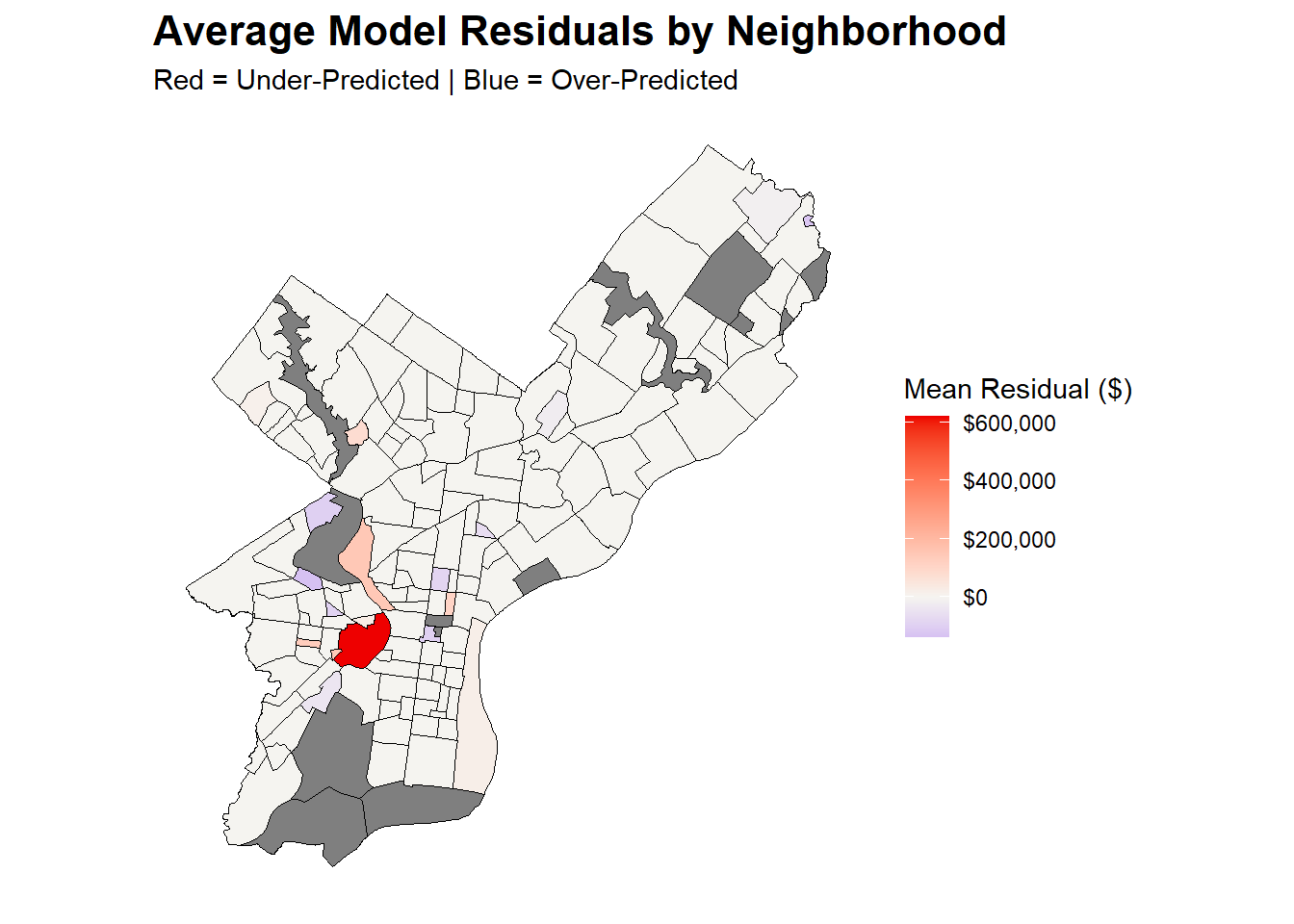
University City is the hardest to predict, Penn owns a lot of property that doesn’t get taxed. And some less wealthy and disinvested neighborhoods are overvalued, like Parkside and Wynnefield in West Philadelphia, but the overall model predicts pretty accurately for most neighborhoods in Philadelphia.

Cross-Validation

10-Fold Cross-Validation

Logged Price Response Variable

library(caret)
# 10-fold cross-validation
# first model
set.seed(0)

train_control <- trainControl(method = "cv", number = 10, savePredictions="final")

cv_log_1 <- train(ln_sale_price ~ ln_square_feet + bath_num + # Structural.
                    ac_binary + fireplace_num + story_num + garage_num + # Structural.
                    basement_type + fuel_type + # Categorical structural.
                    age + I(age^2), # Age polynomial.
                    data = final_data,
                    method = "lm",
                    trControl = train_control)

cv_log_1$results

  intercept      RMSE  Rsquared       MAE      RMSESD RsquaredSD       MAESD
1      TRUE 0.3816682 0.6094278 0.2897425 0.009088709 0.01740783 0.004395093

library(caret)
# 10-fold cross-validation
# second model
set.seed(0)

train_control <- trainControl(method = "cv", number = 10, savePredictions="final")

cv_log_2 <- train(ln_sale_price ~ ln_square_feet + bath_num + # Structural.
                    ac_binary + fireplace_num + story_num + garage_num + # Structural.
                    basement_type + fuel_type + # Categorical structural.
                    age + I(age^2) + # Age polynomial.
                    medhhinc + pct_vacant + pct_single_family, # census
                    data = final_data,
                    method = "lm",
                    trControl = train_control)

cv_log_2$results

  intercept      RMSE  Rsquared       MAE     RMSESD RsquaredSD       MAESD
1      TRUE 0.3102648 0.7419939 0.2299054 0.01217619 0.01899135 0.005887415

library(caret)
# 10-fold cross-validation
# third model
set.seed(0)

train_control <- trainControl(method = "cv", number = 10, savePredictions="final")

cv_log_3 <- train(ln_sale_price ~ ln_square_feet + bath_num + # Structural.
                    ac_binary + fireplace_num + story_num + garage_num + # Structural.
                    basement_type + fuel_type + # Categorical structural.
                    age + I(age^2) + # Age polynomial.
                    medhhinc + pct_vacant + pct_single_family +
                    city_dist_mi + septa_half_mi + ln_park_dist + knn_amenity_mi, # Spatial
                    data = final_data,
                    method = "lm",
                    trControl = train_control)

cv_log_3$results

  intercept      RMSE  Rsquared       MAE     RMSESD RsquaredSD       MAESD
1      TRUE 0.2952488 0.7662942 0.2176894 0.01067494 0.01599652 0.005499245

library(caret)
# 10-fold cross-validation
# third model
set.seed(0)

train_control <- trainControl(method = "cv", number = 10, savePredictions="final")

cv_log_4 <- train(ln_sale_price ~ ln_square_feet + bath_num + # Structural.
                    ac_binary + fireplace_num + story_num + garage_num + # Structural.
                    basement_type + fuel_type + # Categorical structural.
                    age + I(age^2) + # Age polynomial.
                    medhhinc + pct_vacant + pct_single_family +
                    city_dist_mi + septa_half_mi + ln_park_dist + knn_amenity_mi + # Spatial
                    knn_amenity_mi * city_dist_mi + septa_half_mi * city_dist_mi + # Interaction between amenities and downtown distance.
                    neighborhood_fe, # Fixed effect  
                    data = final_data,
                    method = "lm",
                    trControl = train_control)

cv_log_4$results

  intercept      RMSE  Rsquared       MAE     RMSESD RsquaredSD       MAESD
1      TRUE 0.2551879 0.8253801 0.1815212 0.01267003 0.01652301 0.004692818

# Compare all 4 models

## Combine four models：cv_model_1, cv_model_2, cv_model_3, cv_model_4
log_compare <- bind_rows(
  cv_log_1$results %>% 
    mutate(Model = "Model 1: Structural"),
  cv_log_2$results %>% 
    mutate(Model = "Model 2: Structural + Census"),
  cv_log_3$results %>% 
    mutate(Model = "Model 3: Structural + Census + Spatial"),
  cv_log_4$results %>% 
    mutate(Model = "Model 4: Final Model")
) %>%
  select(Model, RMSE, Rsquared, MAE) %>% 
  mutate(across(c(RMSE, Rsquared, MAE), round, 3))

## Plot
log_kable <- kable(log_compare,
                     col.names = c("Model", "RMSE", "R²", "MAE"),
                     caption = "Log Model Performance Comparison (10-Fold Cross-Validation)",
                     digits = 4,
                     format.args = list(big.mark = ",")
) %>%
  kable_styling(latex_options = "striped", full_width = FALSE) %>%
  column_spec(1, bold = TRUE, width = "10cm") %>%
  row_spec(0, color = "#f5f4f0", background = "#ff4100")

log_kable

Log Model Performance Comparison (10-Fold Cross-Validation)

Model	RMSE	R²	MAE
Model 1: Structural	0.382	0.609	0.290
Model 2: Structural + Census	0.310	0.742	0.230
Model 3: Structural + Census + Spatial	0.295	0.766	0.218
Model 4: Final Model	0.255	0.825	0.182

Unlogged Price Response Variable

library(caret)
# 10-fold cross-validation
# first model
set.seed(0)

train_control <- trainControl(method = "cv", number = 10, savePredictions="final")

cv_model_1 <- train(sale_price ~ ln_square_feet + bath_num + # Structural.
                    ac_binary + fireplace_num + story_num + garage_num + # Structural.
                    basement_type + fuel_type + # Categorical structural.
                    age + I(age^2), # Age polynomial.
                    data = final_data,
                    method = "lm",
                    trControl = train_control)

cv_model_1$results

  intercept     RMSE  Rsquared      MAE   RMSESD RsquaredSD    MAESD
1      TRUE 174881.3 0.5946383 102296.6 25555.15 0.06642462 3870.938

library(caret)
# 10-fold cross-validation
# second model
set.seed(0)

train_control <- trainControl(method = "cv", number = 10, savePredictions="final")

cv_model_2 <- train(sale_price ~ ln_square_feet + bath_num + # Structural.
                    ac_binary + fireplace_num + story_num + garage_num + # Structural.
                    basement_type + fuel_type + # Categorical structural.
                    age + I(age^2) + # Age polynomial.
                    medhhinc + pct_vacant + pct_single_family, # census
                    data = final_data,
                    method = "lm",
                    trControl = train_control)

cv_model_2$results

  intercept     RMSE  Rsquared     MAE   RMSESD RsquaredSD    MAESD
1      TRUE 160396.3 0.6588349 88635.4 28556.53 0.07587715 3803.434

library(caret)
# 10-fold cross-validation
# third model
set.seed(0)

train_control <- trainControl(method = "cv", number = 10, savePredictions="final")

cv_model_3 <- train(sale_price ~ ln_square_feet + bath_num + # Structural.
                    ac_binary + fireplace_num + story_num + garage_num + # Structural.
                    basement_type + fuel_type + # Categorical structural.
                    age + I(age^2) + # Age polynomial.
                    medhhinc + pct_vacant + pct_single_family +
                    city_dist_mi + septa_half_mi + ln_park_dist + knn_amenity_mi, # Spatial
                    data = final_data,
                    method = "lm",
                    trControl = train_control)

cv_model_3$results

  intercept     RMSE  Rsquared      MAE   RMSESD RsquaredSD    MAESD
1      TRUE 153234.2 0.6884576 84701.65 28578.51 0.07398629 4072.517

library(caret)
# 10-fold cross-validation
# third model
set.seed(0)

train_control <- trainControl(method = "cv", number = 10, savePredictions="final")

cv_model_4 <- train(sale_price ~ ln_square_feet + bath_num + # Structural.
                    ac_binary + fireplace_num + story_num + garage_num + # Structural.
                    basement_type + fuel_type + # Categorical structural.
                    age + I(age^2) + # Age polynomial.
                    medhhinc + pct_vacant + pct_single_family +
                    city_dist_mi + septa_half_mi + ln_park_dist + knn_amenity_mi + # Spatial
                    knn_amenity_mi * city_dist_mi + septa_half_mi * city_dist_mi + # Interaction between amenities and downtown distance.
                    neighborhood_fe, # Fixed effect  
                    data = final_data,
                    method = "lm",
                    trControl = train_control)

cv_model_4$results

  intercept     RMSE  Rsquared      MAE   RMSESD RsquaredSD    MAESD
1      TRUE 137218.3 0.7496165 72327.67 29554.89 0.07463082 3804.496

# Compare all 4 models

## Combine four models：cv_model_1, cv_model_2, cv_model_3, cv_model_4
model_compare <- bind_rows(
  cv_model_1$results %>% 
    mutate(Model = "Model 1: Structural"),
  cv_model_2$results %>% 
    mutate(Model = "Model 2: Structural + Census"),
  cv_model_3$results %>% 
    mutate(Model = "Model 3: Structural + Census + Spatial"),
  cv_model_4$results %>% 
    mutate(Model = "Model 4: Final Model")
) %>%
  select(Model, RMSE, Rsquared, MAE) %>% 
  mutate(across(c(RMSE, Rsquared, MAE), round, 3))

## Plot
model_kable <- kable(model_compare,
                     col.names = c("Model", "RMSE ($)", "R²", "MAE ($)"),
                     caption = "Model Performance Comparison (10-Fold Cross-Validation)",
                     digits = 4,
                     format.args = list(big.mark = ",")
) %>%
  kable_styling(latex_options = "striped", full_width = FALSE) %>%
  column_spec(1, bold = TRUE, width = "10cm") %>%
  row_spec(0, color = "#f5f4f0", background = "#ff4100")

model_kable

Model Performance Comparison (10-Fold Cross-Validation)

Model	RMSE ($)	R²	MAE ($)
Model 1: Structural	174,881.3	0.595	102,296.64
Model 2: Structural + Census	160,396.3	0.659	88,635.40
Model 3: Structural + Census + Spatial	153,234.2	0.688	84,701.65
Model 4: Final Model	137,218.3	0.750	72,327.67

# Create predicted vs. actual plot

pred_df <- cv_model_4$pred

# Plot Predicted vs Actual 
pred_v_act <- ggplot(pred_df, aes(x = obs, y = pred)) +
  geom_point(alpha = 0.5, color = "#2C7BB6") +
  geom_abline(intercept = 0, slope = 1, color = "red", linetype = "dashed") +
  labs(
    title = "Predicted vs. Actual Sale Price",
    x = "Actual Sale Price ($)",
    y = "Predicted Sale Price ($)"
  ) +
  scale_x_continuous(labels = scales::dollar) +
  scale_y_continuous(labels = scales::dollar) +
  theme_minimal() +
  theme(
    plot.title = element_text(face = "bold", size = 14, margin = margin(b = 10)),
    panel.grid.minor = element_blank(),
    axis.title.x = element_text(margin = margin(t = 10)),
    axis.title.y = element_text(margin = margin(r = 10))
  )

pred_v_act

Model Diagnostics

Check Assumptions

resid_df <- data.frame(
  fitted = fitted(final_model),
  residuals = resid(final_model)
)

resid_v_fit <- ggplot(resid_df, aes(x = fitted, y = residuals)) +
  geom_point(alpha = 0.5, color = "#2C7BB6") +
  geom_hline(yintercept = 0, color = "red", linetype = "dashed") +
  labs(
    title = "Residuals vs. Fitted Values",
    x = "Fitted Values (Predicted Sale Price)",
    y = "Residuals"
  ) +
  scale_x_continuous(labels = scales::dollar) +
  scale_y_continuous(labels = scales::dollar) +
  theme_minimal() +
  theme(
    plot.title = element_text(face = "bold", size = 14, margin = margin(b = 10)),
    panel.grid.minor = element_blank(),
    axis.title.x = element_text(margin = margin(t = 10)),
    axis.title.y = element_text(margin = margin(r = 10))
  )

resid_v_fit

Residuals vs Fitted Values:

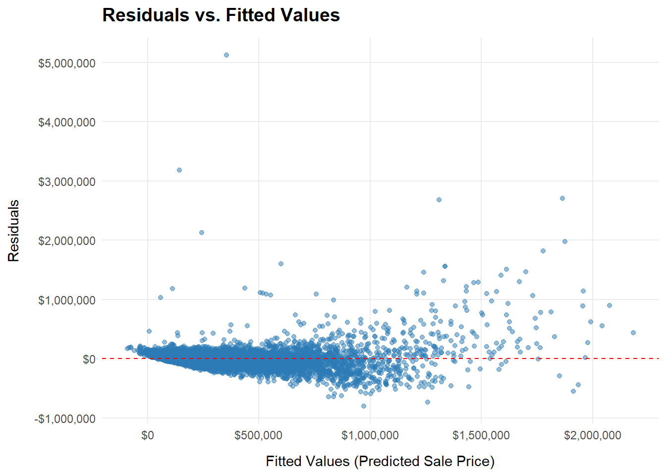
The residual plot shows that most residuals are centered around zero, but the spread of residuals increases as the fitted values grow. This “funnel-shaped” pattern suggests potential heteroskedasticity, meaning the variance of errors may increase for higher-priced properties. While the overall linearity assumption appears reasonable, the increasing dispersion indicates that the model’s prediction error is not constant across the price range.

resid_df <- data.frame(residuals = residuals(final_model))

# Q-Q Plot
qq_plot <- ggplot(resid_df, aes(sample = residuals)) +
  stat_qq(color = "#2C7BB6", alpha = 0.6, size = 2) +      
  stat_qq_line(color = "red", linetype = "dashed") +        
  labs(
    title = "Normal Q-Q Plot of Residuals",
    subtitle = "Check for normality assumption.",
    x = "Theoretical Quantiles (Normal Distribution)",
    y = "Sample Quantiles (Residuals)"
  ) +
  scale_x_continuous(labels = scales::comma) +
  scale_y_continuous(labels = scales::dollar) +
  theme_minimal() +
  theme(
    plot.title = element_text(face = "bold", size = 14, margin = margin(b = 10)),
    plot.subtitle = element_text(size = 11),
    panel.grid.minor = element_blank(),
    axis.title.x = element_text(margin = margin(t = 10)),
    axis.title.y = element_text(margin = margin(r = 10))
  )

qq_plot

Normal Q–Q Plot:

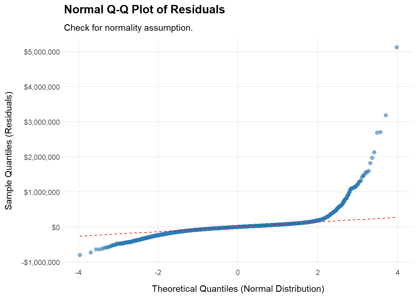
The Q–Q plot reveals that the residuals deviate from the reference line in both tails, especially in the upper tail. This pattern indicates that the residuals are right-skewed and not perfectly normally distributed. The deviation is mainly driven by a small number of very high sale-price observations, which pull the residual distribution upward. However, moderate departures from normality are common in housing price data and generally do not invalidate the model.

cd <- cooks.distance(final_model)

used_row_idx <- as.integer(rownames(model.frame(final_model)))

cooks_df <- tibble(
  row_in_data  = used_row_idx,           
  row_in_model = seq_along(cd),          
  cooks_distance = as.numeric(cd)
)

n_used <- length(cd)
threshold <- 4 / n_used

cooks_plot <- ggplot(cooks_df, aes(x = row_in_model, y = cooks_distance)) +
  geom_bar(stat = "identity", fill = "#2C7BB6", alpha = 0.6) +
  geom_hline(yintercept = threshold, color = "red", linetype = "dashed") +
  coord_cartesian(ylim = c(0, 0.02)) +  
  labs(
    title = "Cook's Distance (Zoomed In)",
    subtitle = paste0("Red Dashed Line = 4/n ≈ ", round(threshold, 5)),
    x = "Observation Index (In-Model)",
    y = "Cook's Distance"
  ) +
  scale_x_continuous(labels = scales::comma) +
  scale_y_continuous(labels = scales::comma) +
  theme_minimal() +
  theme(
    plot.title = element_text(face = "bold", size = 14, margin = margin(b = 10)),
    plot.subtitle = element_text(size = 11),
    panel.grid.minor = element_blank(),
    axis.title.x = element_text(margin = margin(t = 10)),
    axis.title.y = element_text(margin = margin(r = 10))
  )

cooks_plot

# Most influential
top_influential <- cooks_df %>%
  filter(cooks_distance > threshold) %>%
  arrange(desc(cooks_distance)) %>%
  slice_head(n = 10) %>%
  mutate(
    sale_price = final_data$sale_price[row_in_data]   
  ) %>%
  select(row_in_model, row_in_data, sale_price, cooks_distance)

top_influential

# A tibble: 10 × 4
   row_in_model row_in_data sale_price cooks_distance
          <int>       <int>      <dbl>          <dbl>
 1         6038        6038    3600000         0.199 
 2         6307        6307    5477901         0.130 
 3          194         194    3330400         0.0463
 4         8119        8120     480000         0.0457
 5         2467        2467    3995000         0.0400
 6        10355       10356     281000         0.0358
 7         7825        7826     330000         0.0326
 8         2590        2590    3000000         0.0284
 9         1896        1896     170000         0.0238
10         5371        5371    3850000         0.0235

Cook’s Distance:

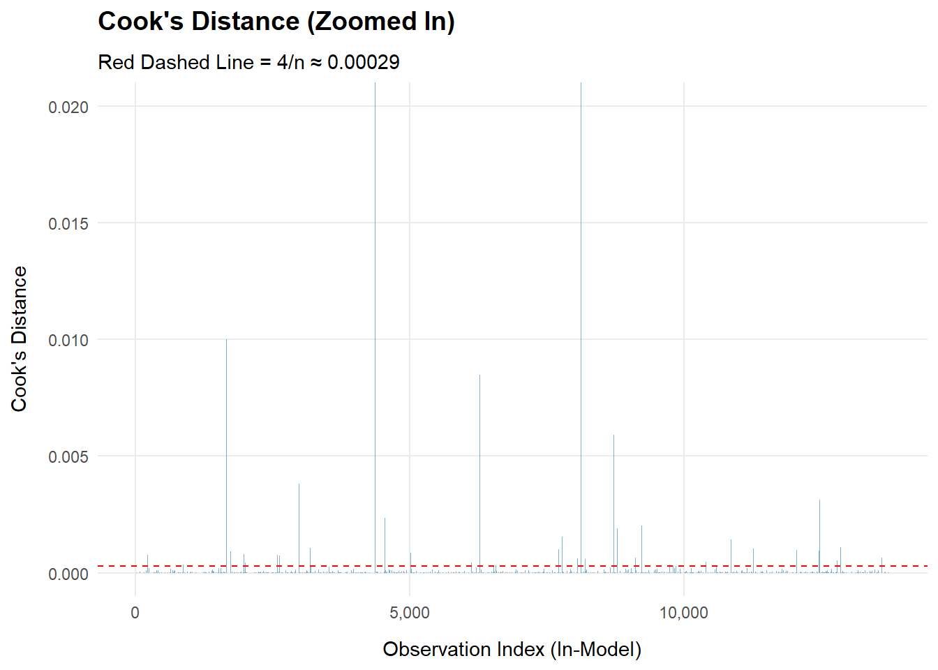
The Cook’s distance plot shows that almost all observations have very small influence values (below the 4/n threshold), indicating that the model is not dominated by a few extreme points. A few cases exhibit slightly higher Cook’s D values, suggesting the presence of mildly influential outliers, but none appear to exert excessive leverage on the regression coefficients.

Detailed Discussion

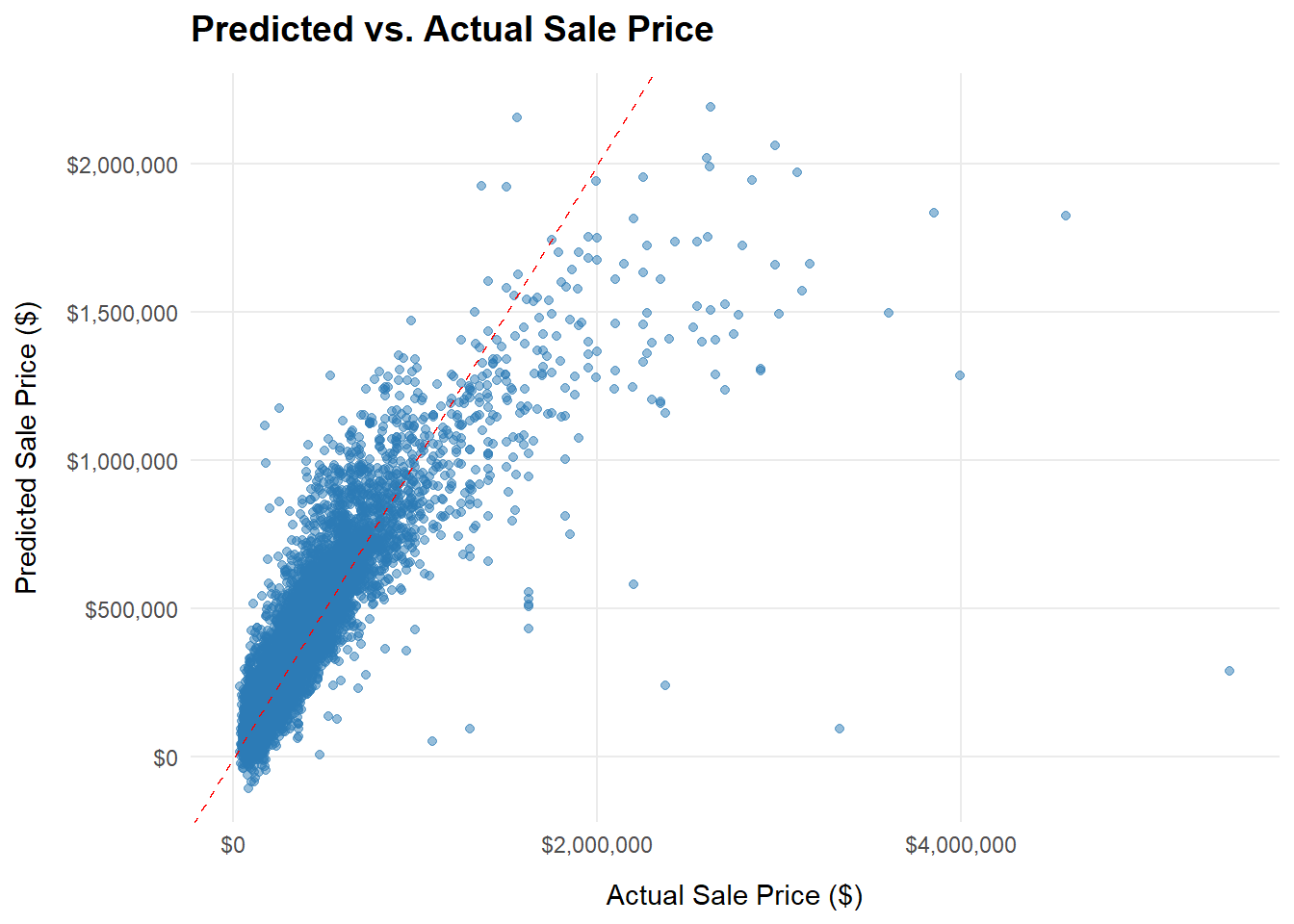
Our final model achieves a cross-validated R² of 0.825, explaining approximately 83% of the variance in Philadelphia residential sale prices. The Mean Absolute Error (MAE) of 72,327.67 USD indicates that, on average, predicted sale prices deviate from actual prices by roughly 17% of the median home price. However, the Root Mean Squared Error (RMSE) of 137,218.70USD—nearly double the MAE—reveals that the model struggles disproportionately with high-value properties. This discrepancy, combined with residuals ranging from about -800,000 USD to +5 million USD, reflects the outsized influence of luxury homes on overall error. Diagnostic plots confirm these patterns: the Q-Q plot shows deviation from normality in both tails (especially the upper tail), while the residuals vs. fitted values plot exhibits a funnel-shaped pattern indicating heteroskedasticity—prediction error variance increases systematically for higher-priced properties. Despite these issues, the median residual of 2,339 USD (near zero) suggests the model’s predictions are generally unbiased for typical homes, and Cook’s distance values remain well below concerning thresholds, indicating no single observation dominates the model.

The model’s minimum and maximum residuals range from about -800,000 USD to +5 million USD, reflecting the outlier influence from luxury properties. While simultaneously referencing the QQ Plot, the model reflects two tails in the plot, but more in the positive region, indicating the model is not 100% normal. However, the residual distribution with the median residual of ~2,300 USD is somewhat marginal in the broader aspect, meaning the model predictions are generally centered about sale prices with limited bias in sale prediction. It is imperative to keep in mind that in the residuals vs fitted values plot, the increase of observations fanning-out as the predicted sale price value increases indicates the existence of heteroskedasticity between some variables.

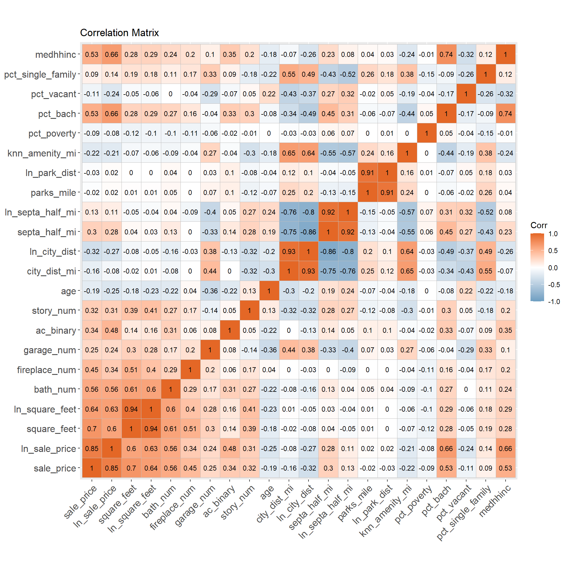
We have concluded that ln_square_feet, neighborhood fixed effects, median household income, number of bathrooms and number of fireplaces as the most significant variables in our model. We calculated this by doing a stepwise regression, and these five yield the highest \(R^2\).

We grossly underpredicted for University City, and a decent amount for Fairmount. This model struggles to accurately predict rural areas and overpredicted uninvested neighborhoods. The severe underprediction of University City may be due to the existence and proximity to Drexel University and the University of Pennsylvania.

External Resources

Downloads

• Property Data

• Neighborhood Boundaries

• Parks

• Tracts Data

• SEPTA Stations

• ACS Data

• Open Street Maps for Points of Interest

Relevant Readings

• Homes in poor neighborhoods are taxed at roughly twice the rate of those in rich areas, study shows

• Philadelphia ranks among top 5 cities for hottest housing market in 2025, Zillow says

• How Major Universities in the US Are Negatively Impacting Local Black Communities

Artificial Intelligence

• Claude: For code debugging in data cleaning and visualizations.

• Chat GPT: For code debugging in data cleaning and visualizations.