Code
# Key Functions
st_filter(data_to_filter, reference_geometry, .predicate = relationship)

# .predicate = ""
st_intersects()
st_touches()
st_within().shp (geometry – lat/long); .dbf (attribute); .sbx (binary spatial index file)Web Mercator (EPSG:3857): Web mapping standard, heavily distorts areas near poles
State Plane / UTM zones: local accuracy, different zones for different regions, optimized for specific geographic areas
Read Spatial Data: st_read
Spatial Subsetting: extract features based on spatial relationships
st_touches looks for neighborsst_withinst_intersects includes the reference feature itself.predicate specified, uses st_intersects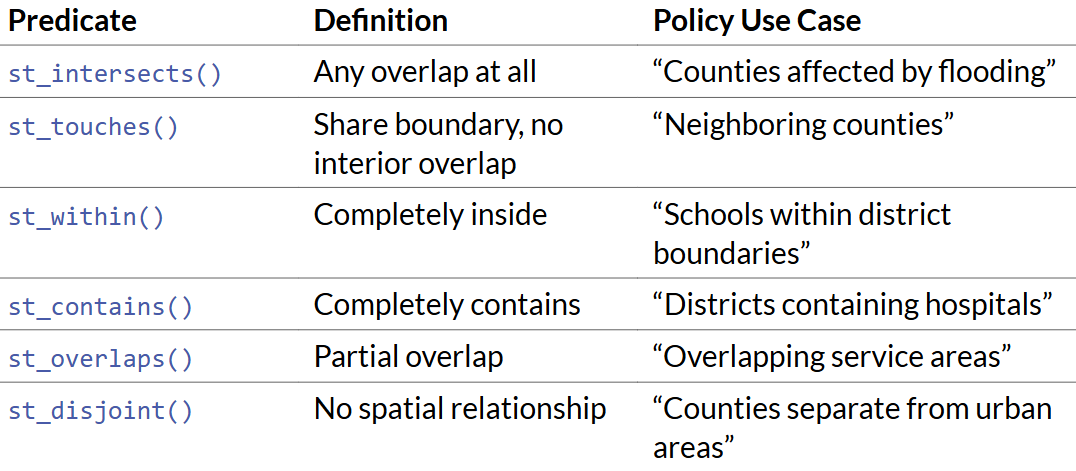
# Key Functions
st_filter(data_to_filter, reference_geometry, .predicate = relationship)
# .predicate = ""
st_intersects()
st_touches()
st_within()Checking and Setting CRS
st_crs(pa_counties)pa_counties <- st_set_crs(pa_counties, 4326)# st_transform
census_tracts <- census_tracts %>%
st_transform(st_crs(pa_counties))
# Transform to Pennsylvania South State Plane (good for PA analysis)
pa_counties_projected <- pa_counties %>% st_transform(crs = 3365)
# Transform to Albers Equal Area (good for area calculations)
pa_counties_albers <- pa_counties %>% st_transform(crs = 5070) `Plot Maps
ggplot(pa_counties) +
  geom_sf() +
  theme_void()
Spatial Joins
tracts_with_counties <- census_tracts %>%
  st_join(pa_counties)
Area Calculations
pa_counties# Convert to Sq Km
pa_counties <- pa_counties %>%
mutate(
area_sqkm = as.numeric(st_area(.)) / 1000000
)Distance and Buffers
# 10km buffer around all hospitals
hospitals_projected <- hospitals %>%
  st_transform(crs = 3365)
st_crs(hospitals_projected)

hospital_buffers <- hospitals_projected %>%
  st_buffer(dist = 32808.4)  # 10,000 meters = 32808.4 feet

ggplot(hospital_buffers)+
  geom_sf()+
  theme_void()

# Different buffer sizes by hospital type (this is hypothetical, we don't have that column!)
hospital_buffers <- hospitals %>%
  mutate(
    buffer_size = case_when(
      type == "Major Medical Center" ~ 15000,
      type == "Community Hospital" ~ 10000,
      type == "Clinic" ~ 5000
    )
  ) %>%
  st_buffer(dist = .$buffer_size)

# Use Unions to calculate what percentage of low-income tracts have access
access_summary <- low_income_tracts %>%
  mutate(
    has_access = st_intersects(., st_union(hospital_buffers), sparse = FALSE)
  ) %>%
  st_drop_geometry() %>%
  summarize(
    total_tracts = n(),
    tracts_with_access = sum(has_access),
    pct_with_access = (tracts_with_access / total_tracts) * 100
  )

print(access_summary)Load data → Get spatial boundaries and attribute data
Check projections → Transform to appropriate CRS
Join datasets → Combine spatial and non-spatial data
Spatial operations → Buffers, intersections, distance calculations
Aggregation → Summarize across spatial units
Visualization → Maps and charts
Interpretation → Policy recommendations
I was surprised at how intuitive and quick it was to develop maps and visualizations using packages in R as compared to ArcGIS. I discussed this with Prof. Delmelle during Office Hours, and she shared that she has relied exclusively on R for the past two years after switching to a Macbook.
While ArcGIS is still a useful tool and has many cool additional features such as StoryMaps or animations, I believe that R is the way forward for core data wrangling, visualization, and machine learning work.