Week 7 Notes - Model Diagnostics and Spatial Autocorrelation

Key Concepts Learned

Regression Workflow

Building the model:

1. Visualize relationships
2. Engineer features
3. Fit the model
4. Evaluate performance (RMSE, R²)
5. Check assumptions

Spatial Diagnostics

6. Are errors random or clustered?
7. Do we predict better in some areas?
8. Is there remaining spatial structure?

Spatial Autocorrelation in Errors (i.e. Clustered Errors)

• spatial pattern visible (not random scatter)
• under/over-predict in areas
• model misses something about location

Moran’s I measures Spatial Autocorrelation

Intuition: When I’m above/below average, are my neighbors also above/below average?

Range: -1 to +1

• +1 = Perfect positive correlation (clustering)
• 0 = Random spatial pattern
• -1 = Perfect negative correlation (dispersion)

---

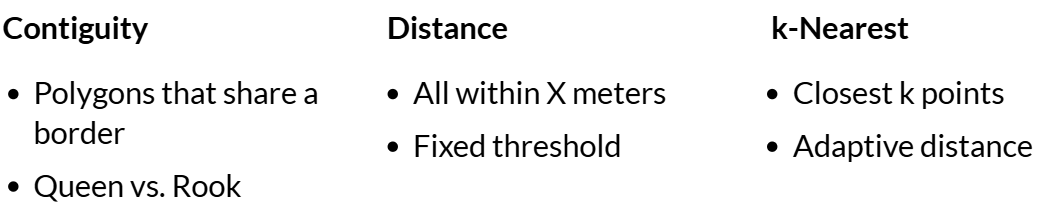
Defining Neighbors:

Sample Example:

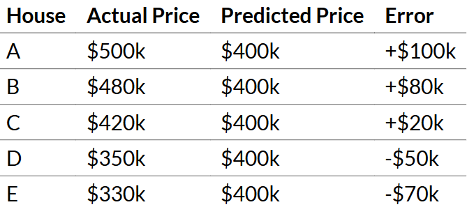
Step 1: Calculate Deviations from Mean

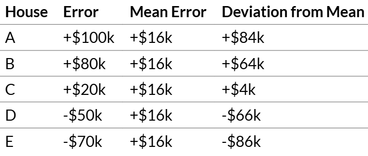
Positive deviation = we over-predicted (actual > predicted)
Negative deviation = we under-predicted (actual < predicted)

Step 2: Multiply Neighbor Pair Deviations

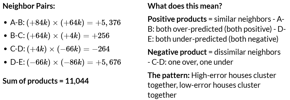
• Lots of positive products → High Moran’s I (clustering)
• Products near zero → Low Moran’s I (random)
• Negative products → Negative Moran’s I (rare with errors)

Step 3: Possible Solutions

If Moran’s I shows clustered errors:

✅ Add more spatial features (different buffers, more amenities)
✅ Try neighborhood fixed effects
✅ Use spatial cross-validation

---

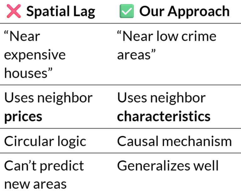
Issues with Spatial Lag for Prediction:

1. Simultaneity Problem (circular logic)

• My price affects neighbors → neighbors affect me
• OLS estimates are biased and inconsistent

2. Prediction Paradox (poor generalizability)

• Need neighbors’ prices to predict my price
• But for new developments or future periods, those prices don’t exist yet

3. Data Leakage in CV

• Spatial Lag “leaks” information from test set
• Artificially good performance that won’t hold

Key Idea: Match method to purpose: 

• inference → spatial lag/error models; prediction → spatial features
• our predicton approach: Instead of modeling dependence in Y (prices), model proximity in X (predictors)

Coding Techniques

• Create and Plot the Spatial Lag

library(spdep)

# Define neighbors (5 nearest)
coords <- st_coordinates(boston_test)
neighbors <- knn2nb(knearneigh(coords, k=5))
weights <- nb2listw(neighbors, style="W")

# Calculate spatial lag of errors
boston_test$error_lag <- lag.listw(weights, boston_test$error)

• Calculate Moran’s I

# Test for spatial autocorrelation in errors
moran_test <- moran.mc(
  boston_test$error,        # Your errors
  weights,                  # Spatial weights matrix
  nsim = 999                # Number of permutations
)

# View results
moran_test$statistic         # Moran's I value

Questions & Challenges

• The intuition behind Moran’s I is “When I’m above/below average, are my neighbors also above/below average?“ I’m curious if incorporating models such as kNN can help to meaningfully reduce spatial lag?

Connections to Policy

• Research methods should follow policy intents and purposes. When looking at market forecasting or policy predictions, the predictive spatial features described above are more useful than spatial econometrics models

Reflection

• I had never heard of Spatial Lag, Spatial Autocorrelation, or Moran’s I before this class as I have not taken spatial statistics, so this was a very useful crash course!