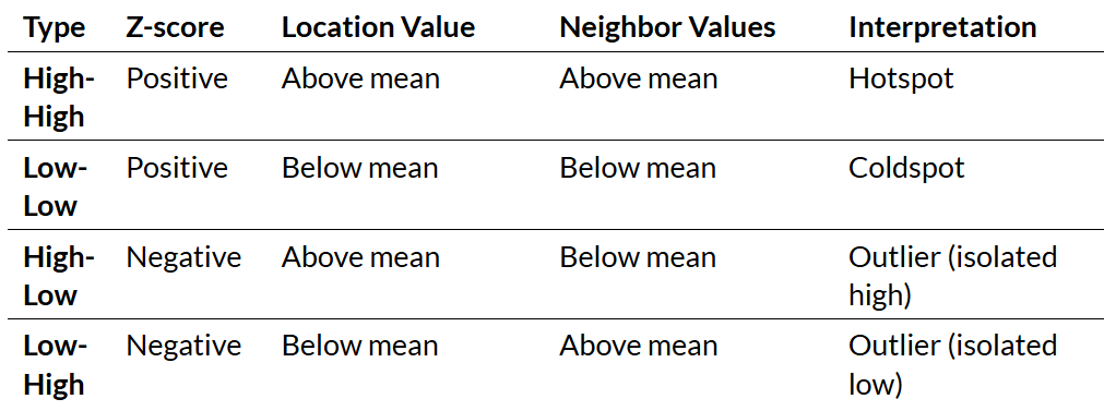
Week 9 Notes - Predictive Policing

Key Concepts Learned

Predictive Policing Sales Pitch

• Efficiency: “Deploy limited resources where they’re needed most”
• Objectivity: “Remove human bias from decision-making”
• Proactivity: “Prevent crime before it happens”
• Data-driven: “Let the data tell us where crime will occur”

Technical Questions

• How do we model crime counts?
• What spatial features predict crime?
• How do we validate predictions?
• Can we outperform baseline methods?

Critical Questions

• Whose data? Whose crimes?
• What if the data is “dirty”? – can we separate “good” from “bad” data?
• Who benefits? Who is harmed?
• What feedback loops are created? – do past patterns predict future crime, or do they just predict policing?
• Can technical solutions fix social problems?

Defining “Dirty Data”

Richardson et al. 2019: “Data derived from or influenced by corrupt, biased, and unlawful practices, including data that has been intentionally manipulated or ‘juked,’ as well as data that is distorted by individual and societal biases.”

1. Fabricated/Manipulated Data – false arrests / downgraded crime classifications
2. Systematically Biased Data – over-policing of certain communities / under-policing of white-collar crime
3. Missing/Incomplete Data – ignored complaints / incomplete reports
4. Proxy Problems – arrests ≠ crimes committed; calls for service ≠ actual need

CautionThe Impossibility of Neutral Crime Data

1. Socially constructed - Societies define what counts as “crime”
2. Selectively enforced - More resources to some neighborhoods
3. Organizationally filtered - Police priorities, department culture
4. Politically shaped - “Tough on crime” eras, moral panics
5. Technically mediated - 911 systems, CAD software, databases

Confirmation Bias Feedback Loop:

• Algorithm learns: “Crime happens in neighborhood X”
• Police sent to neighborhood X
• More arrests in neighborhood X (regardless of actual crime)
• Algorithm “confirmed”: “We were right about neighborhood X!”

Questions to Ask about Any Predictive Policing System

01 | Data Provenance

• What time period does training data cover? What evidence exists that data is accurate?

02 | Variable Selection

• What specific variables are used? How might each variable embed bias?
• What’s excluded and why? Who made these choices?

03 | Validation

• How is accuracy measured? What counts as “success”?
• Are error rates reported by neighborhood?
• Who experiences false positives vs. false negatives?

04 | Deployment

• How do predictions translate to action? What discretion do officers have?

05 | Transparency & Accountability

• Is the methodology public?
• Is there a process to challenge predictions? Who monitors for disparate impact?

06 | Alternatives

• What non-punitive interventions were considered? Could these address root causes instead?

---

Modeling Workflow

01 | Setup & Data Preparation

• Load burglaries (point data)
• Load abandoned cars (311 calls)
• Create fishnet grid (500m × 500m grid)
• Aggregate burglaries to cells

02 | Baseline Comparison

• Kernel Density Estimation (KDE)
• Simple spatial smoothing

03 | Feature Engineering

Using Abandoned Cars as “Disorder Indicator”:

• Count in each cell
• k-Nearest Neighbors (mean distance to 3 nearest)
• LISA (Local Moran’s I - identify hot spots)
• Distance to hot spots (significant clusters)

04 | Count Regression Models

• Fit Poisson regression – test for overdispersion
• Fit Negative Binomial (if overdispersed)
• Interpret coefficients

05 | Spatial Cross-Validation

• Leave-One-Group-Out (LOGO)
• Train on \(n-1\) districts
• Test on held-out district
• Calculate MAE/RMSE

06 | Model Comparison

• Compare to KDE baseline / test both on hold-out data
• Map predictions vs. actual
• Analyze errors spatially

Summary of Different Spatial Measures

• Count → How much disorder is HERE?
• k-NN Distance → How CLOSE are we to disorder?
• Hot Spots (LISA) → Where does disorder CLUSTER?
• Distance to Hot Spots → How close to concentrated disorder?
• Each captures a different aspect of spatial proximity to our indicator variable

Common Approaches to Spatial Weights Matrix (W) – Defining Neighbors

• Contiguity: Share a border? (Queen vs. Rook)
  • Our fishnet grid uses Queen contiguity (most common for regular grids)
  • Row Standardization – Corner Cell with 4 neighbors: each gets weight 0.25 vs Standard Cell with 8 neighbors: each gets weight 0.125
• Distance: Within threshold distance?
• K-nearest neighbors: Closest k locations

Statistical Significance Testing for Moran’s I – Permutation Test

Intuition: only report clusters that are unlikely to occur by chance

1. Calculate observed \(I_i\) for location \(i\)
2. Randomly shuffle values across locations (999 times)
3. Recalculate \(I_i\) for each permutation
4. Compare observed vs. distribution of permuted values
5. If observed is extreme → statistically significant (p < 0.05)

[Four Types of Significant Clusters]

Coding Techniques

• Local Moran’s I – maps showing where patterns/clusters exist

  • numerator: how different is location \(i\) from mean

  • denominator: variance of all locations

  • weight: how different are neighbors from mean

• The Moran Scatterplot

  • x-axis: standardized value at location \(i\)

  • y-axis: spatial lag (weighted average of neighbors)

library(spdep)

# Step 1: Create spatial object
fishnet_sp <- as_Spatial(fishnet)

# Step 2: Define neighbors (Queen contiguity)
neighbors <- poly2nb(fishnet_sp, queen = TRUE)

# Step 3: Create spatial weights (row-standardized)
weights <- nb2listw(neighbors, style = "W", zero.policy = TRUE)

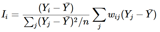
# Step 4: Calculate Local Moran's I
local_moran <- localmoran(
  fishnet$abandoned_cars,  # Variable of interest
  weights,                  # Spatial weights
  zero.policy = TRUE       # Handle cells with no neighbors
)

# Step 5: Extract components
fishnet$local_I <- local_moran[, "Ii"]      # Local I statistic
fishnet$p_value <- local_moran[, "Pr(z != E(Ii))"]  # P-value
fishnet$z_score <- local_moran[, "Z.Ii"]    # Z-score

• Identify & Map Hotspots

# Standardize the variable for quadrant classification
fishnet$standardized_value <- scale(fishnet$abandoned_cars)

# Calculate spatial lag (weighted mean of neighbors)
fishnet$spatial_lag <- lag.listw(weights, fishnet$abandoned_cars)
fishnet$standardized_lag <- scale(fishnet$spatial_lag)

# Identify High-High clusters
fishnet$hotspot <- 0  # Default: not a hotspot

# Criteria: 
# 1. Value above mean (standardized > 0)
# 2. Neighbors above mean (spatial lag > 0)
# 3. Statistically significant (p < 0.05)

fishnet$hotspot[
  fishnet$standardized_value > 0 & 
  fishnet$standardized_lag > 0 & 
  fishnet$p_value < 0.05
] <- 1

# Count hotspots
sum(fishnet$hotspot)

• Distance to Nearest Feature (kNN where k = 1)

  For each grid cell:

  1. Find location of all abandoned cars

  2. Calculate distance to each

  3. Keep minimum distance

library(FNN)

# Calculate distance to nearest abandoned car
nn_dist <- get.knnx(
  data = st_coordinates(abandoned_cars),      # "To" locations
  query = st_coordinates(st_centroid(fishnet)), # "From" locations
  k = 1                                          # Nearest 1
)

# Extract distances
fishnet$abandoned_car_nn <- nn_dist$nn.dist[, 1]

• Distance to Hot Spot

  • Step 1: Identify hotspots (Local Moran’s I High-High clusters)

  • Step 2: distance from each cell to nearest hotspot

# Step 1: Identify hotspots (we did this earlier)
hotspot_cells <- filter(fishnet, hotspot == 1)

# Step 2: Calculate distances
hotspot_dist <- get.knnx(
  data = st_coordinates(st_centroid(hotspot_cells)),
  query = st_coordinates(st_centroid(fishnet)),
  k = 1
)

# Look for concentric patterns around features/hotspots
fishnet$hotspot_nn <- hotspot_dist$nn.dist[, 1]

• Visualizing Distance Features

# Create comparison maps
p1 <- ggplot(fishnet) +
  geom_sf(aes(fill = abandoned_car_nn), color = NA) +
  scale_fill_viridis_c(name = "Distance (m)", option = "plasma") +
  labs(title = "Distance to Nearest Abandoned Car") +
  theme_void()

p2 <- ggplot(fishnet) +
  geom_sf(aes(fill = hotspot_nn), color = NA) +
  scale_fill_viridis_c(name = "Distance (m)", option = "magma") +
  labs(title = "Distance to Nearest Hotspot") +
  theme_void()

grid.arrange(p1, p2, ncol = 2)

---

• Poisson Regression
  • Problem with OLS for Counts: can predict negative values; assumes constant variance; assumes continuous outcome; assumes normal errors
  • Distribution of Crime Counts: right-skewed; many zeros (most cells have no burglaries); discrete (only integer values)
  • Handling Zeros in Count Data: poisson and standard negative binomial typically handles zeros naturally

# Fit Poisson model
model_poisson <- glm(
  countBurglaries ~ Abandoned_Cars + Abandoned_Cars.nn + abandoned.isSig.dist,
  data = fishnet,
  family = poisson(link = "log")
)

# View results
summary(model_poisson)

# Exponentiate coefficients for interpretation
exp(coef(model_poisson))

# Example output:
#                        exp(coef)
# (Intercept)            0.234
# Abandoned_Cars         1.151
# Abandoned_Cars.nn      0.998
# abandoned.isSig.dist   0.999

# Interpretation:
# - Each additional abandoned car → 15.1% increase in expected burglaries
# - Each meter from nearest abandoned car → 0.2% decrease in expected burglaries

• Poisson: Check for Overdispersion
  • Poisson assumption: Variance = Mean
  • Reality with crime data: Variance >> Mean

#  Calculate dispersion parameter
dispersion <- sum(residuals(model_pois, type = "pearson")^2) / 
               model_pois$df.residual

cat("Dispersion parameter:", round(dispersion, 3), "\n")

# Rule of thumb:
# < 1.5: Poisson OK
# 1.5 - 3: Mild overdispersion, NegBin recommended (negative binomial)
# > 3: Serious overdispersion, NegBin essential

• Negative Binomial Regression
  • relaxes the variance = mean assumption

library(MASS)

# Fit Negative Binomial model
model_nb <- glm.nb(
  countBurglaries ~ Abandoned_Cars + Abandoned_Cars.nn + abandoned.isSig.dist,
  data = fishnet
)

# View results
summary(model_nb)

# Compare to Poisson
AIC(model_pois)  # e.g., 8234.5
AIC(model_nb)    # e.g., 6721.3

# Lower AIC = better fit
# If NegBin AIC much lower → use NegBin

# Extract dispersion parameter (theta)
model_nb$theta  # e.g., 2.47

# Interpretation: Significant overdispersion confirmed

• Comparing Poisson vs Negative Binomial

Aspect	Poisson	Negative Binomial
Variance assumption	Var = Mean	Var = μ + αμ²
Overdispersion	Cannot handle	Accommodates
Standard errors	Underestimated if overdispersed	Correctly estimated
When to use	Count data, no overdispersion	Count data with overdispersion
Crime data	Rarely appropriate	Usually better

• Creating a Fishnet Grid

library(sf)

# Step 1: Define cell size (in map units - meters for our projection)
cell_size <- 500  # 500m x 500m cells

# Step 2: Create grid over study area
fishnet <- st_make_grid(
  chicago_boundary,
  cellsize = cell_size,
  square = TRUE,
  what = "polygons"
) %>%
  st_sf() %>%
  mutate(uniqueID = row_number())

# Step 3: Clip to study area (remove cells outside boundary)
fishnet <- fishnet[chicago_boundary, ]

# Check results
nrow(fishnet)  # Number of cells
st_area(fishnet[1, ])  # Area of one cell (should be 250,000 m²)

# Plot Fishnet Pattern
ggplot(fishnet, aes(x = countBurglaries)) +
  geom_histogram(binwidth = 1, fill = "#440154FF", color = "white") +
  labs(
    title = "Distribution of Burglary Counts",
    subtitle = "Most cells have 0-2 burglaries, few have many",
    x = "Burglaries per Cell",
    y = "Number of Cells"
  ) +
  theme_minimal()

• Aggregating Points to Grid

  • Spatial join between crimes (points) and fishnet (polygons)

  • Count crimes per cell

  • Handle cells with zero crimes

# Count burglaries per cell
burglary_counts <- st_join(burglaries, fishnet) %>%
  st_drop_geometry() %>%
  group_by(uniqueID) %>%
  summarize(countBurglaries = n())

# Join back to fishnet
fishnet <- fishnet %>%
  left_join(burglary_counts, by = "uniqueID") %>%
  mutate(countBurglaries = replace_na(countBurglaries, 0))

# Summary
summary(fishnet$countBurglaries)
#   Min. 1st Qu.  Median    Mean 3rd Qu.    Max. 
#      0       0       1    2.3       3      47

• Leave-One-Group-Out (LOGO-CV) Implementation

  • Problem with standard k-fold CV: spatial leakage – model learns from neighbors of test set → overly optimistic performance estimates

  • LOGO-CV: hold out entire spatial groups instead of individual cells

# Get unique districts
districts <- unique(fishnet$District)

# Initialize results
cv_results <- list()

# Loop through districts
for (dist in districts) {
  train_data <- fishnet %>% filter(District != dist)  # Split data
  test_data <- fishnet %>% filter(District == dist)
  
  # Fit model on training data
  model_cv <- glm.nb(
    countBurglaries ~ Abandoned_Cars + Abandoned_Cars.nn + abandoned.isSig.dist,
    data = train_data
  )
  
  # Predict on test data
  test_data$prediction <- predict(model_cv, test_data, type = "response")
  
  # Store results
  cv_results[[dist]] <- test_data
}

# Combine all predictions
all_predictions <- bind_rows(cv_results)

• Common Error Metrics: MAE, RMSE, Mean Error (Bias)

# Calculate metrics by district
cv_metrics <- all_predictions %>%
  group_by(District) %>%
  summarize(
    MAE = mean(abs(countBurglaries - prediction)),
    RMSE = sqrt(mean((countBurglaries - prediction)^2)), 
    ME = mean(countBurglaries - prediction) # negative ME means under-predict
  )

# Map prediction errors
all_predictions <- all_predictions %>%
  mutate(
    error = countBurglaries - prediction,
    abs_error = abs(error),
    pct_error = (prediction - countBurglaries) / (countBurglaries + 1) * 100
  )

# Visualize
ggplot(all_predictions) +
  geom_sf(aes(fill = error), color = NA) +
  scale_fill_gradient2(
    low = "blue", mid = "white", high = "red",
    midpoint = 0,
    name = "Error"
  ) +
  labs(title = "Prediction Errors",
       subtitle = "Red = Over-prediction, Blue = Under-prediction") +
  theme_void()

---

• Calculating Kernel Density Estimation (KDE) as Baseline

library(spatstat)

# Step 1: Convert to point pattern (ppp) object
burglary_ppp <- as.ppp(
  X = st_coordinates(burglaries),
  W = as.owin(st_bbox(chicago_boundary))
)

# Step 2: Calculate KDE
kde_surface <- density.ppp(
  burglary_ppp,
  sigma = 1000,  # Bandwidth in meters (standard in literature)
  edge = TRUE    # Edge correction
)

# Step 3: Extract values to fishnet cells
fishnet$kde_risk <- raster::extract(
  raster(kde_surface),
  st_centroid(fishnet)
)

# Standardize to 0-1 scale for comparison
fishnet$kde_risk <- (fishnet$kde_risk - min(fishnet$kde_risk, na.rm=T)) / 
                     (max(fishnet$kde_risk, na.rm=T) - min(fishnet$kde_risk, na.rm=T))

• Creating Risk Categories

# Create quintiles (5 equal groups)
fishnet$model_risk_category <- cut(
  fishnet$prediction,
  breaks = quantile(fishnet$prediction, probs = seq(0, 1, 0.2)),
  labels = c("1st (Lowest)", "2nd", "3rd", "4th", "5th (Highest)"),
  include.lowest = TRUE
)

fishnet$kde_risk_category <- cut(
  fishnet$kde_risk,
  breaks = quantile(fishnet$kde_risk, probs = seq(0, 1, 0.2)),
  labels = c("1st (Lowest)", "2nd", "3rd", "4th", "5th (Highest)"),
  include.lowest = TRUE
)

• Visualizing Model vs KDE Performance

# Bar chart comparing methods
comparison_data <- bind_rows(
  model_results %>% mutate(Method = "Negative Binomial Model"),
  kde_results %>% mutate(Method = "Kernel Density")
)

ggplot(comparison_data, aes(x = risk_category, y = pct_of_total, fill = Method)) +
  geom_bar(stat = "identity", position = "dodge") +
  scale_fill_manual(values = c("#440154FF", "#FDE724FF")) +
  labs(
    title = "Percentage of 2018 Burglaries Captured",
    subtitle = "Which method performs better in high-risk areas?",
    x = "Risk Category",
    y = "% of Total 2018 Burglaries"
  ) +
  theme_minimal() +
  theme(legend.position = "bottom")

• Procedure for Testing on Hold-Out Data (i.e. data the model has never seen)

  • Train model on 2017 data

  • Create risk predictions for all cells

  • Load 2018 burglaries (new data)

  • Count how many 2018 burglaries fall in each risk category

  • Compare model vs. KDE

Questions & Challenges

• There’s a lot to digest today – I will need to review this material slowly and apply the underlying intuitions to the lab assignment

Connections to Policy

Reflection

• Further Reading: https://www.wired.com/story/how-peter-thiels-secretive-data-company-pushed-into-policing/
• https://blog.palantir.com/about-palantir-ddddb78aec29