Week 10 Notes - Logistic Regression for Binary Outcomes

Key Concepts Learned

Logistic Regression – Binary Classification Problems in Policy

• Criminal Justice: Will someone reoffend? (recidivism) Will someone appear for court? (flight risk)
• Health: Will patient develop disease? (risk assessment) Will treatment be successful? (outcome prediction)
• Economics: Will loan default? (credit risk) Will person get hired? (employment prediction)
• Urban Planning: Will building be demolished? (blight prediction) Will household participate in program? (uptake prediction)

Fundamental Challenge: Threshold

• Cost of false positives (e.g. marking legitimate email as spam)
• Cost of false negatives (e.g. missing actual spam)

Confusion Matrix

• Sensitivity (Recall, True Positive Rate): \[ = \frac{TP}{TP + FN}\]
  • “Of all actual positives, how many did we catch?” / “Sense the sick”
  • False Positive Rate = 1 - Specificity
• Specificity (True Negative Rate): \[ = \frac{TN}{TN + FP}\]
  • “Of all actual negatives, how many did we correctly identify?” / “Spare the healthy”
• Precision (Positive Predictive Value): \[ = \frac{TP}{TP + FP}\]
  • “Of all our positive predictions, how many were correct?”
• Accuracy: \[= \frac{TP + TN}{TP + FP + TN + FN}\]

Disparate Impact & Algorithmic Bias in Action

A model can be “accurate” overall but perform very differently across groups. Group B experiences:

• Lower sensitivity (more people who will reoffend are missed)
• Lower specificity (more people who won’t reoffend are flagged)
• Higher false positive rate (more unjust interventions)

Group	Sensitivity	Specificity	False Positive Rate
Overall	0.72	0.68	0.32
Group A	0.78	0.74	0.26
Group B	0.64	0.58	0.42

Framework for Threshold Selection

Step 1: Understand the consequences

What happens with a false positive? What happens with a false negative? Are costs symmetric or asymmetric?

Step 2: Consider stakeholder perspectives

Who is affected by each type of error? Do all groups experience consequences equally?

Step 3: Choose your metric priority

Maximize sensitivity? (catch all positives) Maximize specificity? (minimize false alarms) Balance precision and recall? (F1 score) Equalize across groups?

Step 4: Test multiple thresholds

Evaluate performance across thresholds Look at group-wise performance Consider sensitivity analysis

---

Coding Techniques

• Example: Email Spam Detection

  • number of exclamation marks

  • contains the word “free”

  • email length

# Create example spam detection data
set.seed(123)
n_emails <- 1000

spam_data <- data.frame(
  exclamation_marks = c(rpois(100, 5), rpois(900, 0.5)),  # Spam has more !
  contains_free = c(rbinom(100, 1, 0.8), rbinom(900, 1, 0.1)),  # Spam mentions "free"
  length = c(rnorm(100, 200, 50), rnorm(900, 500, 100)),  # Spam is shorter
  is_spam = c(rep(1, 100), rep(0, 900))
)

# Fit logistic regression
spam_model <- glm(
  is_spam ~ exclamation_marks + contains_free + length,
  data = spam_data,
  family = "binomial"  # This specifies logistic regression
)

# View results
summary(spam_model)
coefs <- coef(spam_model)
odds_ratios <- exp(coefs)
print(odds_ratios)

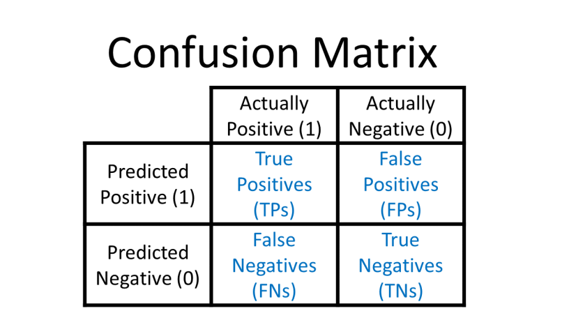
• Confusion Matrix

# Create example predictions
set.seed(123)
spam_data <- data.frame(
  actual_spam = c(rep(1, 100), rep(0, 900)),
  predicted_prob = c(rnorm(100, 0.7, 0.2), rnorm(900, 0.3, 0.2))
) %>%
  mutate(predicted_prob = pmax(0.01, pmin(0.99, predicted_prob)))

# With threshold = 0.5
spam_data <- spam_data %>%
  mutate(predicted_spam = ifelse(predicted_prob > 0.5, 1, 0))

# Calculate confusion matrix
conf_mat <- confusionMatrix(
  as.factor(spam_data$predicted_spam),
  as.factor(spam_data$actual_spam),
  positive = "1"
)

• Threshold Choice

# Calculate metrics at different thresholds
thresholds <- seq(0.1, 0.9, by = 0.1)

metrics_by_threshold <- map_df(thresholds, function(thresh) {
  preds <- ifelse(spam_data$predicted_prob > thresh, 1, 0)
  cm <- confusionMatrix(as.factor(preds), as.factor(spam_data$actual_spam), 
                        positive = "1")
  
  data.frame(
    threshold = thresh,
    sensitivity = cm$byClass["Sensitivity"],
    specificity = cm$byClass["Specificity"],
    precision = cm$byClass["Precision"]
  )
})

# Visualize the trade-off
ggplot(metrics_by_threshold, aes(x = threshold)) +
  geom_line(aes(y = sensitivity, color = "Sensitivity"), size = 1.2) +
  geom_line(aes(y = specificity, color = "Specificity"), size = 1.2) +
  geom_line(aes(y = precision, color = "Precision"), size = 1.2) +
  labs(title = "The Threshold Trade-off",
       subtitle = "As threshold increases, we become more selective",
       x = "Probability Threshold", y = "Metric Value") +
  theme_minimal() +
  theme(legend.position = "bottom")

• ROC Curve

  • Goal: illustrate trade-off between true positive rate and false positive rate

  • X-axis: False Positive Rate (1 - Specificity)

  • Y-axis: True Positive Rate (Sensitivity)

# Create ROC curve for our spam example
roc_obj <- roc(spam_data$actual_spam, spam_data$predicted_prob)

# Plot it
ggroc(roc_obj, color = "steelblue", size = 1.2) +
  geom_abline(slope = 1, intercept = 1, linetype = "dashed", color = "gray50") +
  labs(title = "ROC Curve: Spam Detection Model",
       subtitle = paste0("AUC = ", round(auc(roc_obj), 3)),
       x = "1 - Specificity (False Positive Rate)",
       y = "Sensitivity (True Positive Rate)") +
  theme_minimal() +
  coord_fixed()

# Print AUC
auc_value <- auc(roc_obj)
cat("\nArea Under the Curve (AUC):", round(auc_value, 3))

Interpreting AUC

• AUC = 1.0: Perfect classifier
• AUC = 0.9-1.0: Excellent
• AUC = 0.8-0.9: Good
• AUC = 0.7-0.8: Acceptable

Questions & Challenges

• Private-sector software providers may be very hesitant to publicly share the inner workings and metrics of their predictive algorithms

Connections to Policy – Practical Recommendations

1. Report multiple metrics - not just accuracy
2. Show the ROC curve - demonstrates trade-offs
3. Test multiple thresholds - document your choice
4. Evaluate by sub-group - check for disparate impact
5. Document assumptions - explain why you chose your threshold
6. Consider context - what are the real-world consequences?
7. Provide uncertainty - confidence intervals, not just point estimates
8. Enable recourse - can predictions be challenged?

Reflection

• Further Reading: https://www.washingtonpost.com/news/monkey-cage/wp/2016/10/17/can-an-algorithm-be-racist-our-analysis-is-more-cautious-than-propublicas/