Philadelphia Housing Price Prediction - Technical Appendix
Author
Nina Carlsen, Ryan Drake, Sujanesh Kakumanu, Kavana Raju, Chloe Robinson, Henry Sywulak-Herr.
This technical appendix documents the full workflow used to engineer and visualize spatial features for predicting residential housing prices in Philadelphia.
We apply several filters to the property data to for quality and relevance. First, we restrict our analysis to residential properties sold between 2023 and 2024, excluding any other property categories. Second, we remove properties with sale prices below $10, as these are abnormal prices for residential properties.
To work with Github file size limits, the data is further trimmed of irrelevant columns.
Code
# Restrict to residential onlyresidential_categories <-c("APARTMENTS > 4 UNITS","MULTI FAMILY","SINGLE FAMILY","MIXED USE")residential_data <- sf_data %>%filter(category_code_description %in% residential_categories,year(sale_date) %in%c(2023, 2024), mailing_city_state =="PHILADELPHIA PA", sale_price >10 )table(residential_data$category_code_description)# Making sure the file saved to the repo is the trimmed data (to stay below GitHub data limits)st_write(residential_data, "./data/OPA_data.geojson", driver ="GeoJSON", delete_dsn =TRUE, quiet =TRUE)file.exists("./data/OPA_data.geojson")OPA_raw <-st_read("./data/OPA_data.geojson", quiet =TRUE) %>%st_transform(2272)# OPA_data -> cutting mostly NA columns or irrelevant columns for this model.OPA_raw <- OPA_raw %>%select(-c( cross_reference, date_exterior_condition, exempt_land, fireplaces, fuel, garage_type, house_extension, mailing_address_2, mailing_care_of, market_value_date, number_of_rooms, other_building, owner_2, separate_utilities, sewer, site_type, street_direction, suffix, unfinished, unit, utility ))names(OPA_raw)
The property sales data was gathered from the OPA properties public data set from the City of Philadelphia. This data set was 32 columns and 583,825 observations. This file was too large for our shared GitHub work space so it was reduced by filtering for residential properties, years 2023 and 2024, location within Philadelphia, and sale price over 10 since some were NA, 1, or 10. This was just enough to get the most basic and general data to work with that ran with GitHub size limits. This reduced the size to 22121 observations. The original geojson file was overwritten and named OPA_data.
Properties selected for residential included apartments >4 units, single family, multi-family, and mixed use. Mixed use was left in as there are still residential unit to account yet add more complex property types to our total data set when comparing sale price and other aspects such as total area to other observations. These properties should also be cross referenced with zoning codes for future research.
We left mixed use in during this process to give us the most general data set representation. There was also limited data cleaning other than omitting columns that were mostly NA. This gave our model the most general data set to work with despite lower future RMSE values. Future research would be needed to most accurately assess the choices of losing data and a more generalized Philadelphia housing market verses very clean data and more specific Philadelphia housing market that may omit certain aspects of the housing market like data in lower income areas or multi use residential aspects. This could have also been conducted in grouping NA values and sparse categories. More complexity could be accounted for in future work.
This was our start simple and add complexity approach. Our original to final OPA data set went from 583,825 to 22,121 observations and from 32 to 68 variables.
1.2 Exploratory Data Analysis
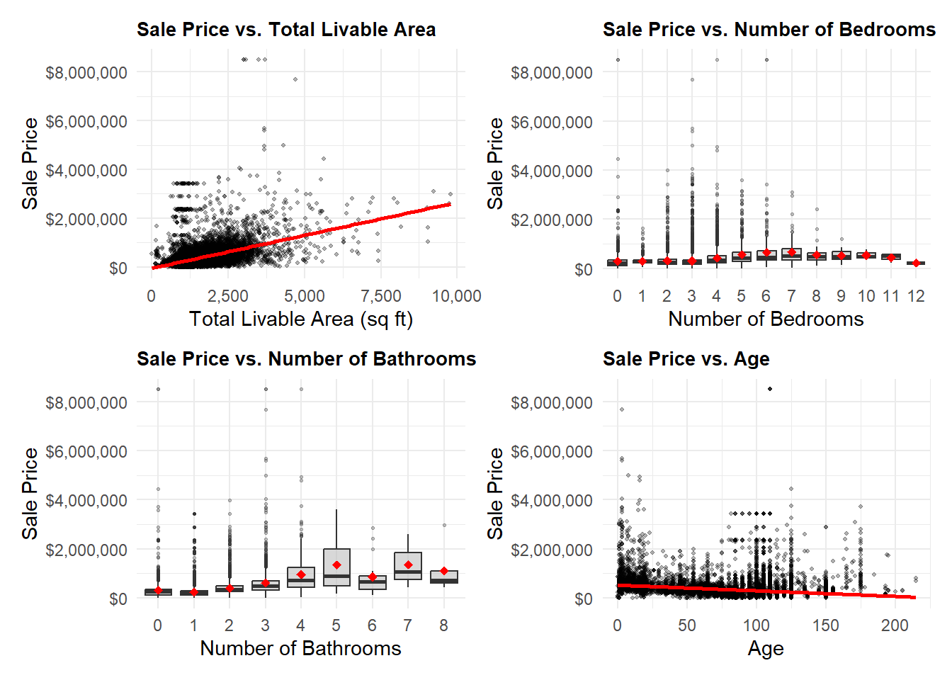
Below are selected property variables—Total Livable Area, Bedrooms, Bathrooms, and Age—in relation to Sale Price. Properties with excessive square footage (>10,000 sqft), missing bedroom or bathroom data, over 12 bathrooms with low sale prices, or implausible construction years were removed to reduce skew and data errors. This additional filtering was kept for the rest of the analysis in this report.
Code
# filter out outliers from the datasetOPA_data <- OPA_raw %>%filter( total_livable_area <=10000, year_built >1800,!is.na(number_of_bathrooms),!is.na(number_of_bedrooms), number_of_bathrooms <12, ) %>%mutate(year_built =as.numeric(year_built),building_age =2025- year_built )p1 <-ggplot(OPA_data, aes(x = total_livable_area, y = sale_price)) +geom_point(alpha =0.3, size =0.8) +geom_smooth(method ="lm", color ="red", se =TRUE) +scale_y_continuous(labels =dollar_format()) +scale_x_continuous(labels =comma_format()) +labs(title ="Sale Price vs. Total Livable Area",x ="Total Livable Area (sq ft)",y ="Sale Price" ) +theme_minimal() +theme(plot.title =element_text(size =10, face ="bold"))p2 <-ggplot(OPA_data, aes(x =factor(number_of_bedrooms), y = sale_price)) +geom_boxplot(fill ="gray", alpha =0.6, outlier.alpha =0.3, outlier.size =0.5) +stat_summary(fun = mean, geom ="point", color ="red", size =2, shape =18) +scale_y_continuous(labels =dollar_format()) +labs(title ="Sale Price vs. Number of Bedrooms",x ="Number of Bedrooms",y ="Sale Price" ) +theme_minimal() +theme(plot.title =element_text(size =10, face ="bold"))p3 <-ggplot(OPA_data, aes(x =factor(number_of_bathrooms), y = sale_price)) +geom_boxplot(fill ="gray", alpha =0.6, outlier.alpha =0.3, outlier.size =0.5) +stat_summary(fun = mean, geom ="point", color ="red", size =2, shape =18) +scale_y_continuous(labels =dollar_format()) +labs(title ="Sale Price vs. Number of Bathrooms",x ="Number of Bathrooms",y ="Sale Price" ) +theme_minimal() +theme(plot.title =element_text(size =10, face ="bold"))p4 <-ggplot(OPA_data, aes(x = building_age, y = sale_price)) +geom_point(alpha =0.3, size =0.8) +geom_smooth(method ="lm", color ="red", se =TRUE) +scale_y_continuous(labels =dollar_format()) +labs(title ="Sale Price vs. Age",x ="Age",y ="Sale Price" ) +theme_minimal() +theme(plot.title =element_text(size =10, face ="bold"))# Combine plots(p1 | p2) / (p3 | p4)
`geom_smooth()` using formula = 'y ~ x'
`geom_smooth()` using formula = 'y ~ x'
1.3 Feature Engineering
Code
OPA_data <- OPA_data %>%mutate(# convert to numeric before interactionstotal_livable_area =as.numeric(total_livable_area),census_tract =as.numeric(as.character(census_tract)),year_built =as.numeric(year_built),total_area =as.numeric(total_area),market_value =as.numeric(market_value),number_of_bedrooms =as.numeric(number_of_bedrooms),# building code and total areaint_type_tarea =as.numeric(as.factor(building_code_description)) * total_area,# market and livable areaint_value_larea = market_value * total_livable_area,# market and total areaint_value_tarea = market_value * total_area,# livable area and exterior conditionint_larea_econd = total_livable_area *as.numeric(as.factor(exterior_condition)),# livable area and interior conditionint_larea_icond = total_livable_area *as.numeric(as.factor(interior_condition)),# livable area and bedroomsint_larea_beds = total_livable_area * number_of_bedrooms )
Code
pa_crs <-2272neighbor_points <-st_transform(OPA_data, pa_crs)nrow(nhoods)st_crs(neighbor_points)nhoods <-st_transform(nhoods, 2272)#joining houses to neighborhoodsneighbor_points <- neighbor_points %>%st_join(., nhoods, join = st_intersects)# one property doesn't lie in any neighborhoodneighbor_points <- neighbor_points[!is.na(neighbor_points$NAME),]#results neighbor_points %>%st_drop_geometry() %>%count(NAME) %>%arrange(desc(n))
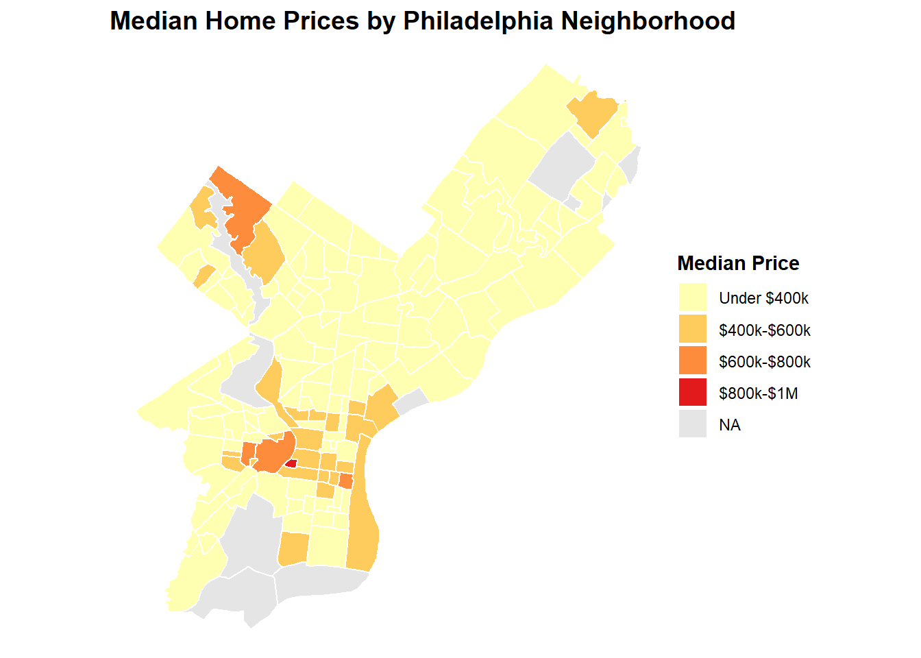
# Define wealthy as >=$420,000 which is 1.5x city median of 279,900nhoods_prices <- nhoods_prices %>%mutate(wealthy_neighborhood =ifelse(median_price >=420000, "Wealthy", "Not Wealthy"),wealthy_neighborhood =as.factor(wealthy_neighborhood) )nhoods_prices %>%st_drop_geometry() %>%count(wealthy_neighborhood)
  wealthy_neighborhood   n
1          Not Wealthy 123
2              Wealthy  26
3                 <NA>  10
Code
neighbor_points <- neighbor_points %>%left_join(., nhoods_prices %>% st_drop_geometry %>%select(NAME, wealthy_neighborhood),by ="NAME")# Still add neighbor points to OPA data
Households were denoted as wealthy if their median household price was over $420,000, which is 1.5x city median of 279,900. This term will be used in an interaction in Model 4 to account for theoretical differences in wealthy neighborhoods, such as inflated costs for additional home amenities such as bedrooms, bathrooms, or livable floor area.
2 Census Data
2.1 Data Preparation
Code
# link variables and aliasesvars <-c("pop_tot"="B01001_001","med_hh_inc"="B19013_001","med_age"="B01002_001")# the FIPS code for the state of PA is 42fips_pa <-42
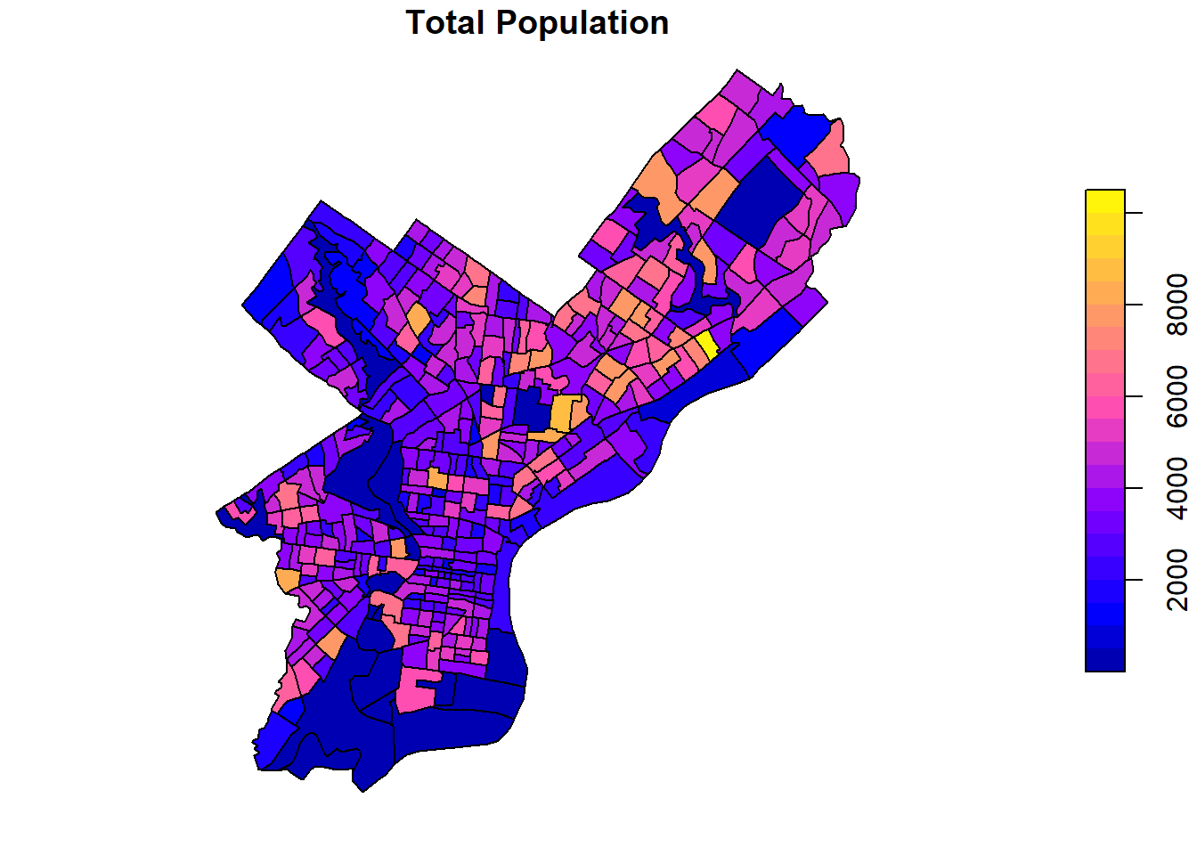
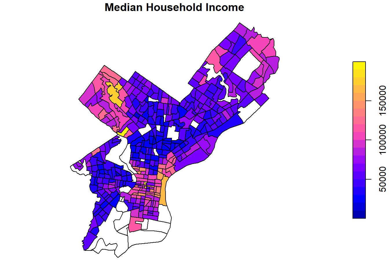
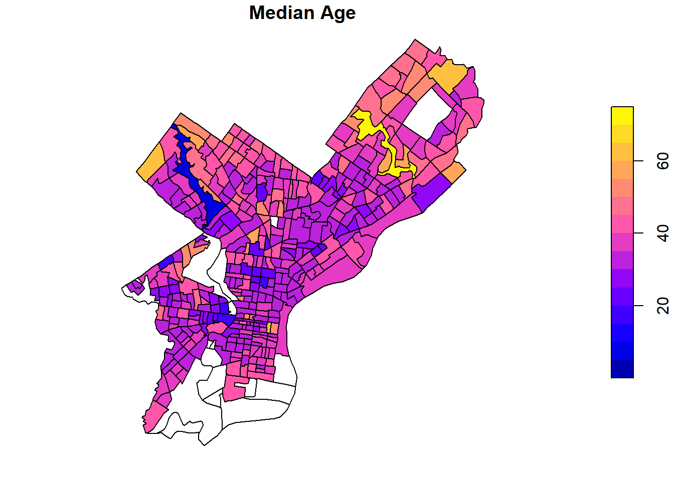
Variables pulled from the census include total population, median household income, and median age.
Code
# retrieve data from the ACS for 2023demo_vars_pa <-get_acs(geography ="tract",variable = vars,year =2023,state = fips_pa,output ="wide",geometry = T,progress_bar = F) %>%st_transform(2272)# separate NAME column into its constituent partsdemo_vars_pa <- demo_vars_pa %>%separate(NAME,into =c("TRACT", "COUNTY", "STATE"),sep ="; ",remove = T) %>%mutate(TRACT =parse_number(TRACT),COUNTY =sub(x = COUNTY, " County", ""))# filter out Philadelphia tractsdemo_vars_phl <- demo_vars_pa %>%filter(COUNTY =="Philadelphia")
# get NA counts per columnna_counts <-sapply(demo_vars_phl, function(x) {sum(is.na(x))})kable(t(as.data.frame(na_counts)))
GEOID
TRACT
COUNTY
STATE
pop_totE
pop_totM
med_hh_incE
med_hh_incM
med_ageE
med_ageM
geometry
na_counts
0
0
0
0
0
0
27
27
17
17
0
Code
# filter out all rows that have at least one column with an na valuena_index <-!complete.cases(demo_vars_phl %>%st_drop_geometry())demo_vars_phl_na <- demo_vars_phl[na_index,]kable(head(demo_vars_phl_na, 5) %>%select(-ends_with("M")) %>%st_drop_geometry(),col.names =c("GeoID", "Tract", "County", "State", "Population", "Median HH Inc ($)", "Median Age (yrs)"),row.names = F)
GeoID
Tract
County
State
Population
Median HH Inc ($)
Median Age (yrs)
42101016500
165.00
Philadelphia
Pennsylvania
2165
NA
44.1
42101980902
9809.02
Philadelphia
Pennsylvania
0
NA
NA
42101980800
9808.00
Philadelphia
Pennsylvania
0
NA
NA
42101028500
285.00
Philadelphia
Pennsylvania
2625
NA
36.1
42101036901
369.01
Philadelphia
Pennsylvania
49
NA
42.1
27 and 17 census tracts have a value of NA for median household income and median age, respectively. For the 17 census tracts where there is no reported population, the median household income and median age will be set to 0. The remaining 10 census tracts that have population but no reported median household income will be omitted from the dataset.
Code
# create a dataset with NAs replaced with zero where applicabledemo_vars_phl_rep <- demo_vars_phl %>%mutate(med_hh_incE =case_when(pop_totE ==0&is.na(med_hh_incE) ~0,.default = med_hh_incE),med_ageE =case_when(pop_totE ==0&is.na(med_ageE) ~0,.default = med_ageE))# final cleaned dataset without the 10 census tracts that have population values but have NA values for Median Household Incomedemo_vars_phl_clean <- demo_vars_phl_rep[complete.cases(demo_vars_phl_rep %>%select(-ends_with("M")) %>%st_drop_geometry()),]# table with the omitted census tractsdemo_vars_phl_omit <- demo_vars_phl_rep[!complete.cases(demo_vars_phl_rep %>%select(-ends_with("M")) %>%st_drop_geometry()),]kable(demo_vars_phl_omit %>%select(-ends_with("M")) %>%st_drop_geometry(),col.names =c("GeoID", "Tract", "County", "State", "Population", "Median HH Inc ($)", "Median Age (yrs)"),row.names = F, caption ="Census Tracts Omitted from Analysis due to Data Unavailability")
Census Tracts Omitted from Analysis due to Data Unavailability
GeoID
Tract
County
State
Population
Median HH Inc ($)
Median Age (yrs)
42101016500
165.00
Philadelphia
Pennsylvania
2165
NA
44.1
42101028500
285.00
Philadelphia
Pennsylvania
2625
NA
36.1
42101036901
369.01
Philadelphia
Pennsylvania
49
NA
42.1
42101014800
148.00
Philadelphia
Pennsylvania
892
NA
40.9
42101027700
277.00
Philadelphia
Pennsylvania
5489
NA
36.9
42101030100
301.00
Philadelphia
Pennsylvania
6446
NA
37.2
42101989100
9891.00
Philadelphia
Pennsylvania
1240
NA
29.7
42101989300
9893.00
Philadelphia
Pennsylvania
160
NA
30.5
42101020500
205.00
Philadelphia
Pennsylvania
3383
NA
33.3
42101980200
9802.00
Philadelphia
Pennsylvania
396
NA
74.9
Code
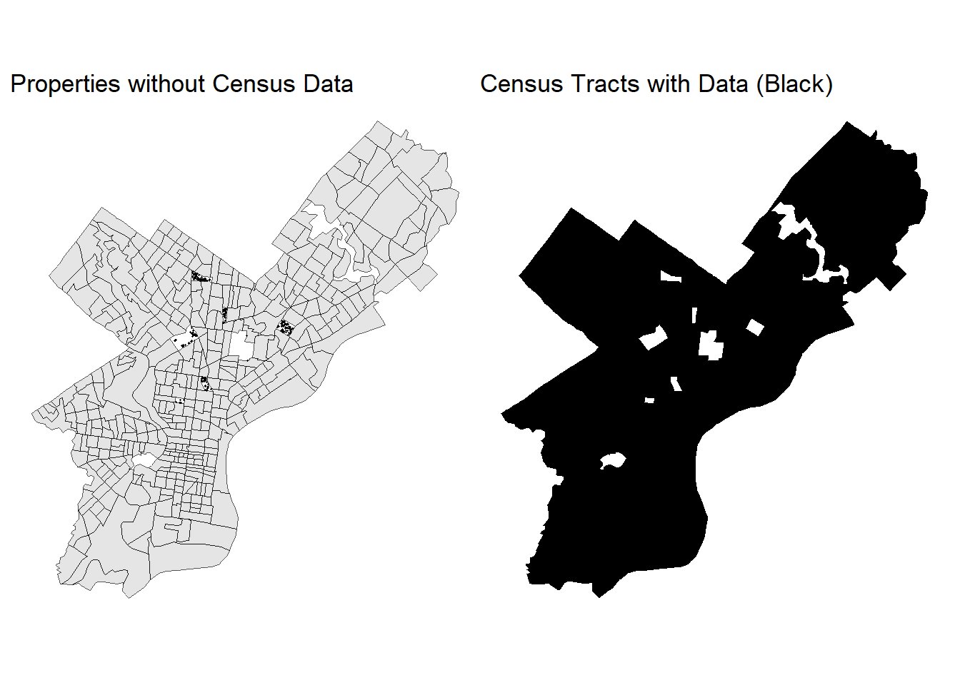
# join census variables to the OPA dataOPA_data <-st_join(OPA_data, demo_vars_phl_clean %>%select(pop_totE, med_hh_incE, med_ageE))# isolate NA rows and plot where they arecensusNAs <- OPA_data[is.na(OPA_data$med_hh_incE),]census_plt1 <-ggplot() +geom_sf(data = demo_vars_phl_clean$geometry) +geom_sf(data = censusNAs, size =0.15) +theme_void() +labs(title ="Properties without Census Data")census_plt2 <-ggplot() +geom_sf(data = demo_vars_phl_clean$geometry, fill ="black", color ="transparent") +theme_void() +labs(title ="Census Tracts with Data (Black)")(census_plt1 | census_plt2)
Of the 22121 properties in the dataset after cleaning and omitting outliers, 248 - approximately 1.1% of the dataset - have no associated census data due to the lack of a Median Household Income value for those census tracts. Comparing plots of property locations without census data and that of census tracts which have data confirms this spatial relationship.
3 Spatial Features
3.1 Data Preparation
This stage prepares and validates the OpenDataPhilly spatial datasets used to engineer neighborhood-level variables for the housing model.
Steps Performed
Transformed all spatial datasets to EPSG 2272 (NAD83 / PA South ftUS) for consistent distance measurements.
Removed invalid geometries, dropped Z/M values, and converted all housing geometries to points.
Imported and projected OpenDataPhilly amenities:
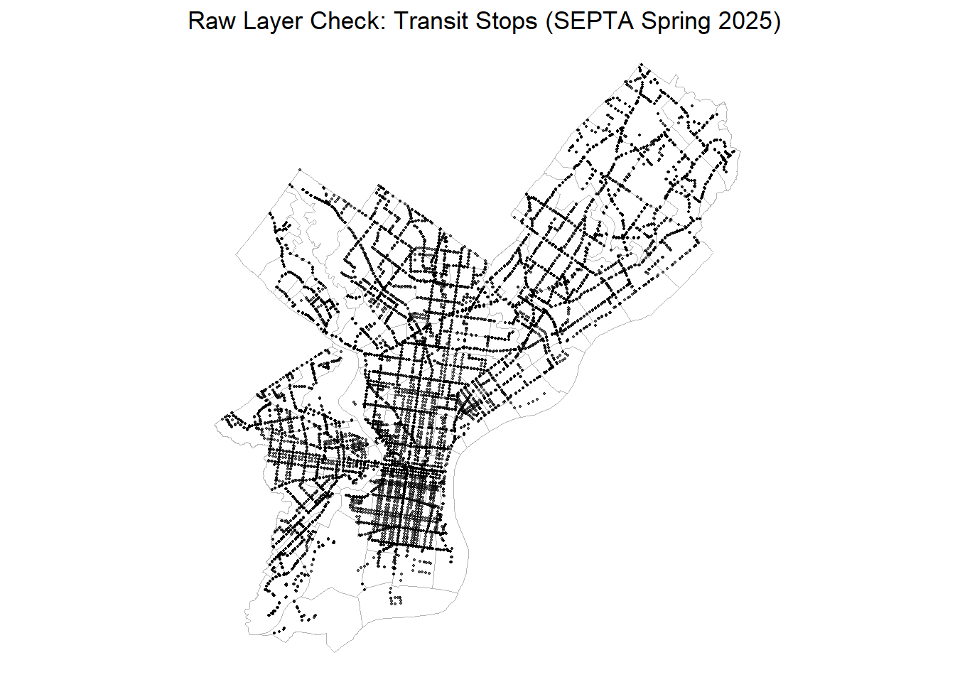
Transit Stops
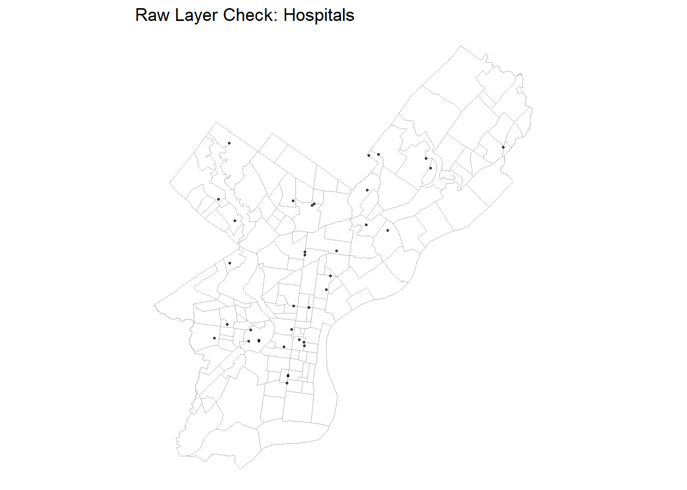
Hospitals
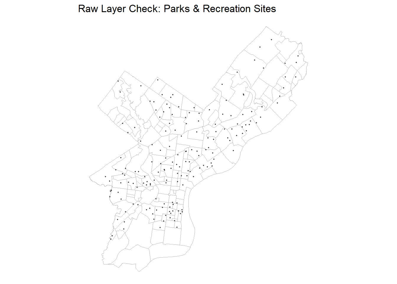
Parks & Recreation Sites
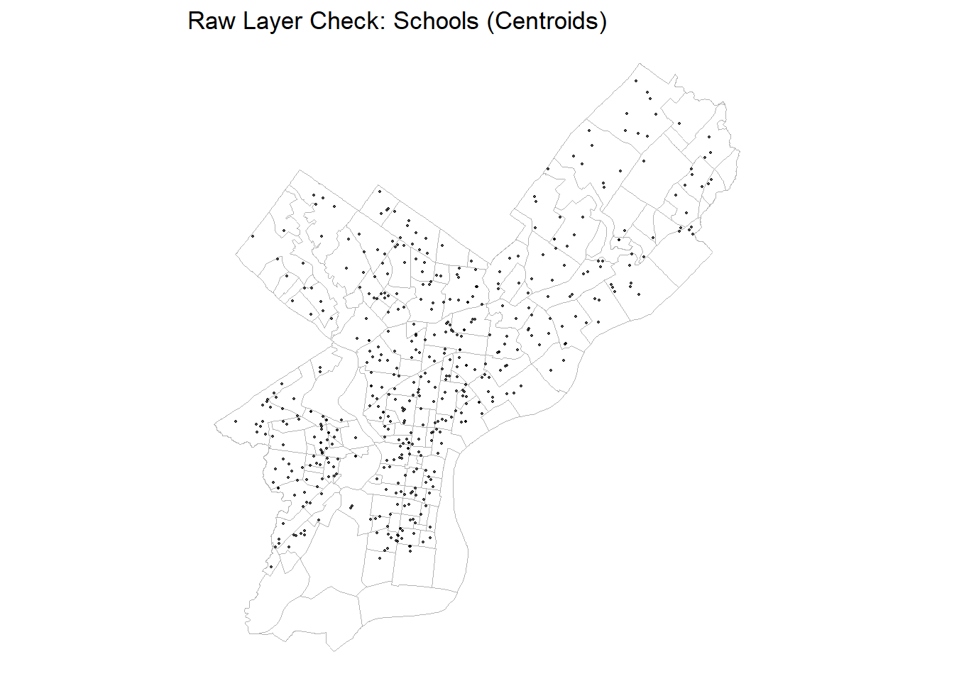
Schools Parcels (centroids created from polygon features)
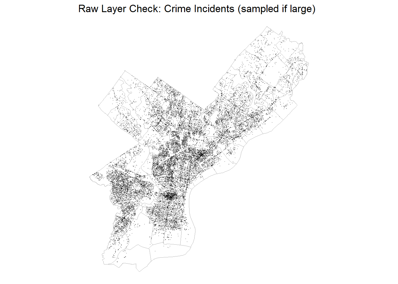
Crime Incidents (2023 and 2024 combined)
Code
#CRS & radiipa_crs <-2272# NAD83 / PA South (ftUS)mi_to_ft <-5280r_park_ft <-0.25* mi_to_ftr_crime_ft <-0.50* mi_to_ftr_school_ft <-0.50* mi_to_ft# turn off spherical geometry (makes buffer/join ops faster)sf::sf_use_s2(FALSE)## CONVERT SALES DATA TO POINTS ##OPA_points <-st_transform(OPA_data, pa_crs)#Drop Z/M if presentst_geometry(OPA_points) <-st_zm(st_geometry(OPA_points), drop =TRUE, what ="ZM")#Make geometries validst_geometry(OPA_points) <-st_make_valid(st_geometry(OPA_points))#Ensure POINT geometry (works for points/lines/polygons/collections)st_geometry(OPA_points) <-st_point_on_surface(st_geometry(OPA_points))#Add sale IDOPA_points <- OPA_points %>%mutate(sale_id = dplyr::row_number())#read & project layerstransit <-st_read("./data/Transit_Stops_(Spring_2025)/Transit_Stops_(Spring_2025).shp", quiet =TRUE) |>st_transform(pa_crs)hospitals <-st_read("./data/Hospitals.geojson", quiet =TRUE) |>st_transform(pa_crs)parksrec <-st_read("./data/PPR_Program_Sites.geojson", quiet =TRUE)|>st_transform(pa_crs)schools_polygons <-st_read("./data/Schools_Parcels.geojson", quiet =TRUE) |>st_transform(pa_crs)crime_2023 <-st_read("./data/crime_incidents_2023/incidents_part1_part2.shp", quiet =TRUE) |>st_transform(pa_crs)crime_2024 <-st_read("./data/crime_incidents_2024/incidents_part1_part2.shp", quiet =TRUE) |>st_transform(pa_crs)#combine 2023 & 2024 crime datasetscrime <-rbind(crime_2023, crime_2024)#create centroids for schools datasetschools <-if (any(st_geometry_type(schools_polygons) %in%c("POLYGON","MULTIPOLYGON"))) {st_centroid(schools_polygons, )} else { schools_polygons}#crop transit data to philadelphiaphilly_boundary <-st_union(nhoods)transit <-st_filter(transit, philly_boundary, .predicate = st_within)
3.2 Exploratory Data Analysis
Exploratory plots and maps examine the raw accessibility patterns across Philadelphia before feature engineering.
Code
# Transit stops (raw)ggplot() +geom_sf(data = nhoods, fill =NA, color ="grey70", linewidth =0.3) +geom_sf(data = transit, size =0.3, alpha =0.6) +labs(title ="Raw Layer Check: Transit Stops (SEPTA Spring 2025)") +theme_void()
# Parks & Recreation Program Sites (raw)ggplot() +geom_sf(data = nhoods, fill =NA, color ="grey70", linewidth =0.3) +geom_sf(data = parksrec, size =0.4, alpha =0.6) +labs(title ="Raw Layer Check: Parks & Recreation Sites") +theme_void()
Code
# Schools (centroids of polygons) — rawggplot() +geom_sf(data = nhoods, fill =NA, color ="grey70", linewidth =0.3) +geom_sf(data = schools, size =0.4, alpha =0.7) +labs(title ="Raw Layer Check: Schools (Centroids)") +theme_void()
Code
# Crime points are huge; sampling for speedset.seed(5080)crime_quick <-if (nrow(crime) >30000) dplyr::slice_sample(crime, n =30000) else crimeggplot() +geom_sf(data = nhoods, fill =NA, color ="grey70", linewidth =0.3) +geom_sf(data = crime_quick, size =0.1, alpha =0.25) +labs(title ="Raw Layer Check: Crime Incidents (sampled if large)") +theme_void()
3.2.1 Interpretation
Transit Stops: Dense corridors radiate from Center City, showing strong transit coverage.
Hospitals: Sparse but geographically balanced.
Parks & Recreation: uneven distribution,
Schools: evenly distributed across most neighborhoods
Crime: Visibly concentrated, confirming the need for log-transformed counts
3.3 Feature Engineering
Spatial features were derived using two complementary approaches: k-Nearest Neighbor (kNN) and buffer-based counts, depending on whether accessibility was best captured as proximity or exposure.
# feature 3 - parks/rec sites within 0.25 mi (count)rel_parks <- sf::st_is_within_distance(OPA_points, parksrec, dist = r_park_ft)OPA_points <- OPA_points %>%mutate(parks_cnt_0p25mi =lengths(rel_parks))# feature 4 - crime count within 0.5 mi (per square mile)crime_buffer <-st_buffer(OPA_points, dist = r_crime_ft)rel_crime <-st_intersects(crime_buffer, crime, sparse =TRUE)# count number of crimescrime_cnt <-lengths(rel_crime)rm(rel_crime)OPA_points <- OPA_points |>mutate(crime_cnt_0p5mi = crime_cnt,log1p_crime_cnt_0p5 =log1p(crime_cnt_0p5mi) )# feature 5 - schools within 0.5 mi (using centroids)rel_sch <- sf::st_is_within_distance(OPA_points, schools, dist = r_school_ft)OPA_points <- OPA_points %>%mutate(schools_cnt_0p5mi =lengths(rel_sch))
3.3.1 Summary Table and Justification
Feature
Method
Parameter
Theoretical Rationale
Distance to Nearest Transit Stop
kNN (k = 1)
–
Captures ease of access to public transport; nearest stop approximates walkability and job access.
Distance to Nearest Hospital
kNN (k = 1)
–
Reflects accessibility to health care and emergency services; proximity adds perceived security for households.
Parks & Rec Sites within 0.25 mi
Buffer Count
r = 0.25 mi
Measures exposure to green space and recreational facilities within a 5-minute walk; positive amenity effect on property value.
Crime Incidents within 0.5 mi
Buffer Count
r = 0.5 mi
Represents local safety environment; higher crime counts reduce housing desirability.
Schools within 0.5 mi
Buffer Count
r = 0.5 mi
Reflects educational access and family appeal; clustering of schools often raises residential demand.
Population
Census
–
Represents the present residential demand within a census tract
Median Household Income
Census
–
Indicative of the ability of present residents of a census tract to afford housing
Median Age
Census
–
Measure of the dominant age group in a census tract (i.e. high student or elderly population)
3.3.2 Feature Validation and Visualization
Code
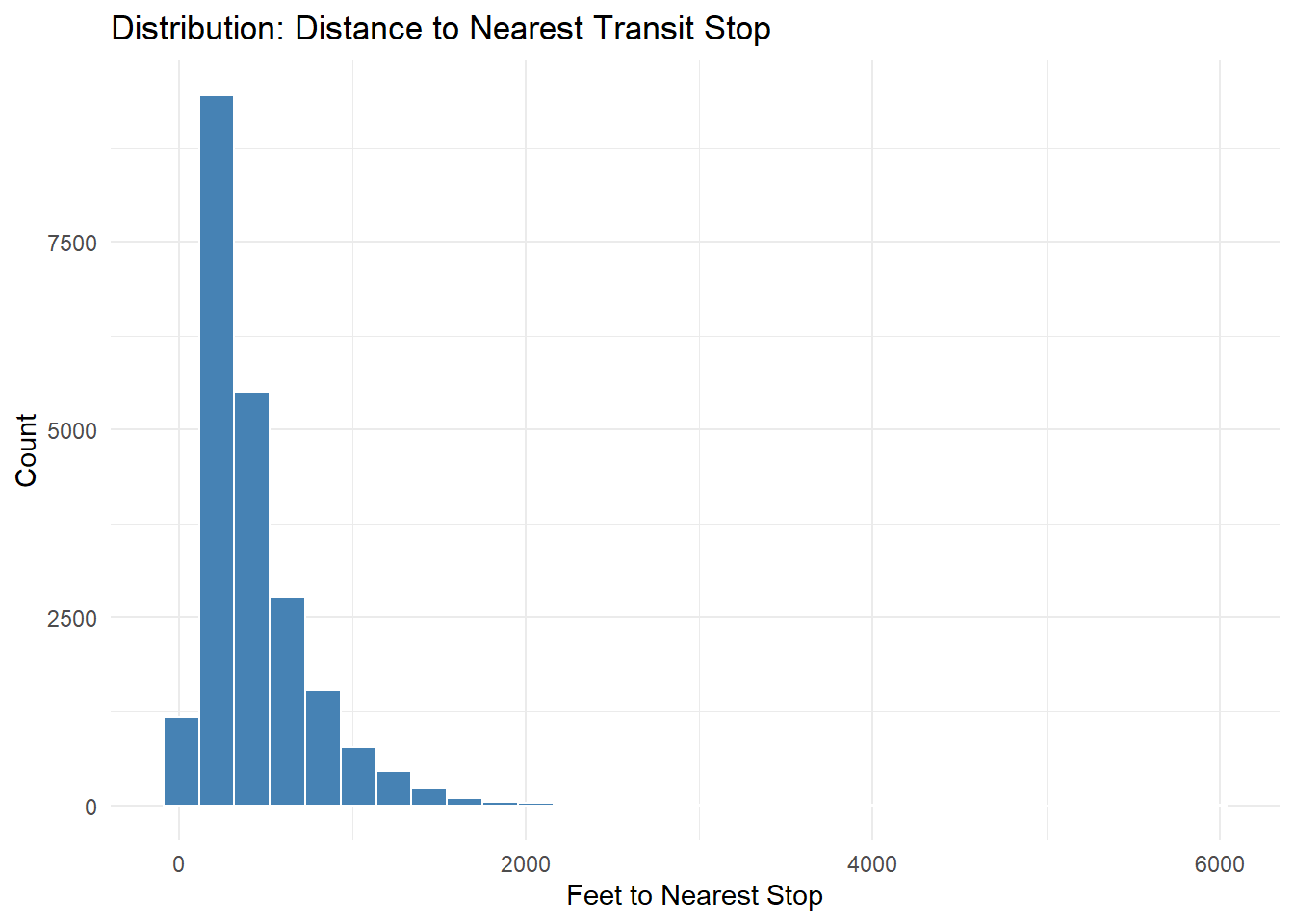
## Transit Accessibilityggplot(OPA_points, aes(x = dist_nearest_transit_ft)) +geom_histogram(fill ="steelblue", color ="white", bins =30) +labs(title ="Distribution: Distance to Nearest Transit Stop",x ="Feet to Nearest Stop", y ="Count") +theme_minimal()
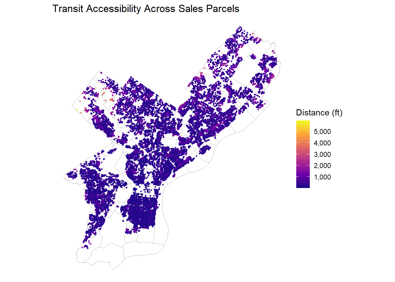
Code
ggplot(OPA_points) +geom_sf(data = nhoods, fill =NA, color ="grey70", linewidth =0.3) +geom_sf(aes(color = dist_nearest_transit_ft), size =0.5) +scale_color_viridis_c(option ="plasma", labels = comma) +labs(title ="Transit Accessibility Across Sales Parcels",color ="Distance (ft)") +theme_void()
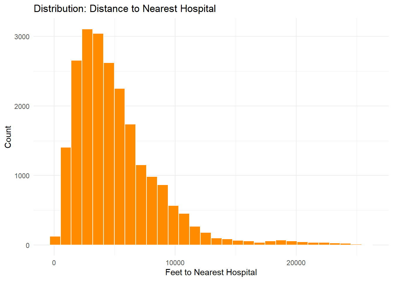
Code
## Hospital Proximityggplot(OPA_points, aes(x = dist_nearest_hospital_ft)) +geom_histogram(fill ="darkorange", color ="white", bins =30) +labs(title ="Distribution: Distance to Nearest Hospital",x ="Feet to Nearest Hospital", y ="Count") +theme_minimal()
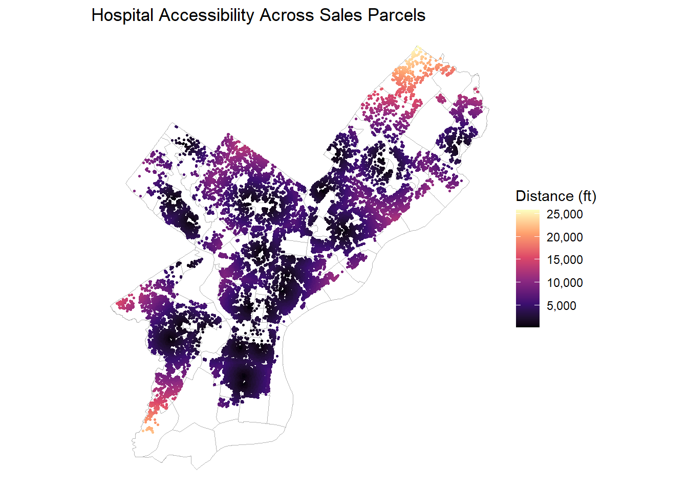
Code
ggplot(OPA_points) +geom_sf(data = nhoods, fill =NA, color ="grey70", linewidth =0.3) +geom_sf(aes(color = dist_nearest_hospital_ft), size =0.5) +scale_color_viridis_c(option ="magma", labels = comma) +labs(title ="Hospital Accessibility Across Sales Parcels",color ="Distance (ft)") +theme_void()
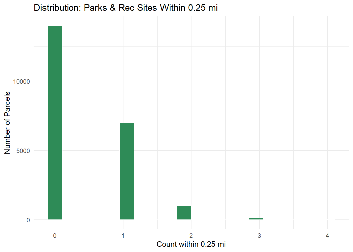
Code
## Parks & Recreationggplot(OPA_points, aes(x = parks_cnt_0p25mi)) +geom_histogram(fill ="seagreen", color ="white", bins =20) +labs(title ="Distribution: Parks & Rec Sites Within 0.25 mi",x ="Count within 0.25 mi", y ="Number of Parcels") +theme_minimal()
Code
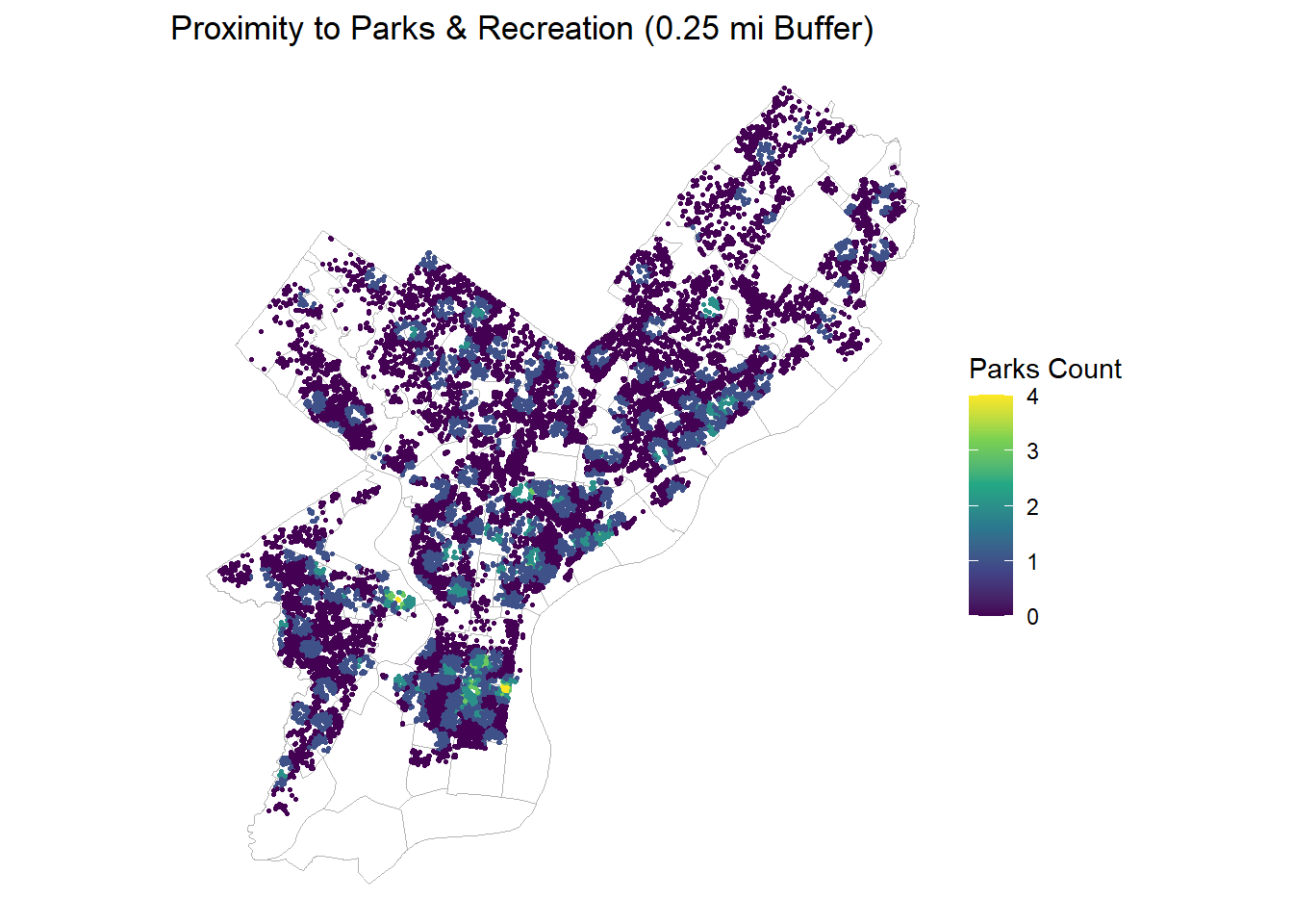
ggplot(OPA_points) +geom_sf(data = nhoods, fill =NA, color ="grey70", linewidth =0.3) +geom_sf(aes(color = parks_cnt_0p25mi), size =0.6) +scale_color_viridis_c(option ="viridis") +labs(title ="Proximity to Parks & Recreation (0.25 mi Buffer)",color ="Parks Count") +theme_void()
Code
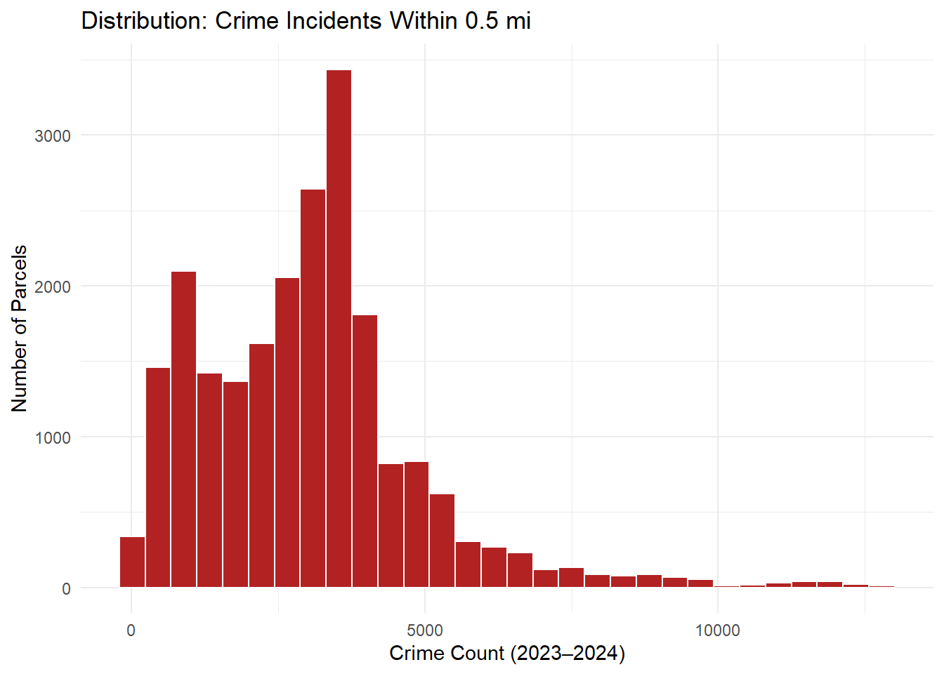
## Crime Countsggplot(OPA_points, aes(x = crime_cnt_0p5mi)) +geom_histogram(fill ="firebrick", color ="white", bins =30) +labs(title ="Distribution: Crime Incidents Within 0.5 mi",x ="Crime Count (2023–2024)", y ="Number of Parcels") +theme_minimal()
Code
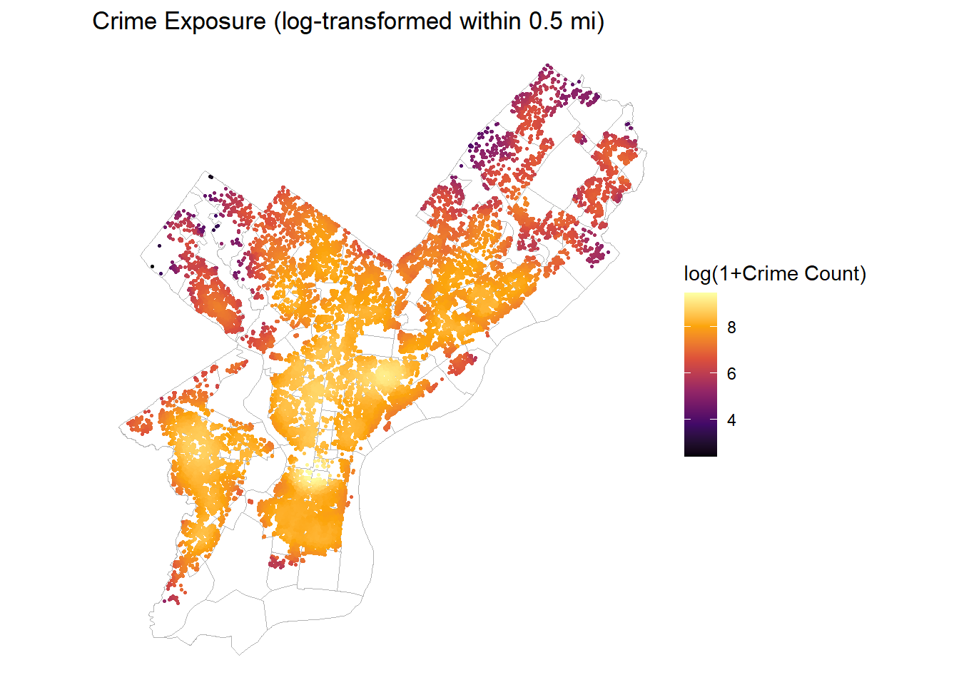
ggplot(OPA_points) +geom_sf(data = nhoods, fill =NA, color ="grey70", linewidth =0.3) +geom_sf(aes(color = log1p_crime_cnt_0p5), size =0.6) +scale_color_viridis_c(option ="inferno") +labs(title ="Crime Exposure (log-transformed within 0.5 mi)",color ="log(1+Crime Count)") +theme_void()
Code
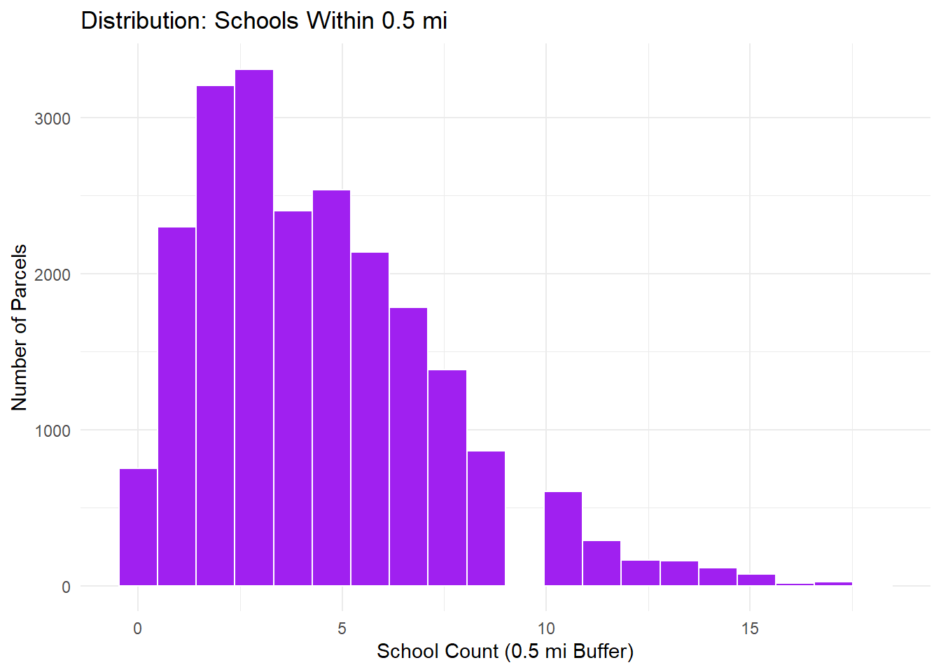
## Schools Accessibilityggplot(OPA_points, aes(x = schools_cnt_0p5mi)) +geom_histogram(fill ="purple", color ="white", bins =20) +labs(title ="Distribution: Schools Within 0.5 mi",x ="School Count (0.5 mi Buffer)", y ="Number of Parcels") +theme_minimal()
Code
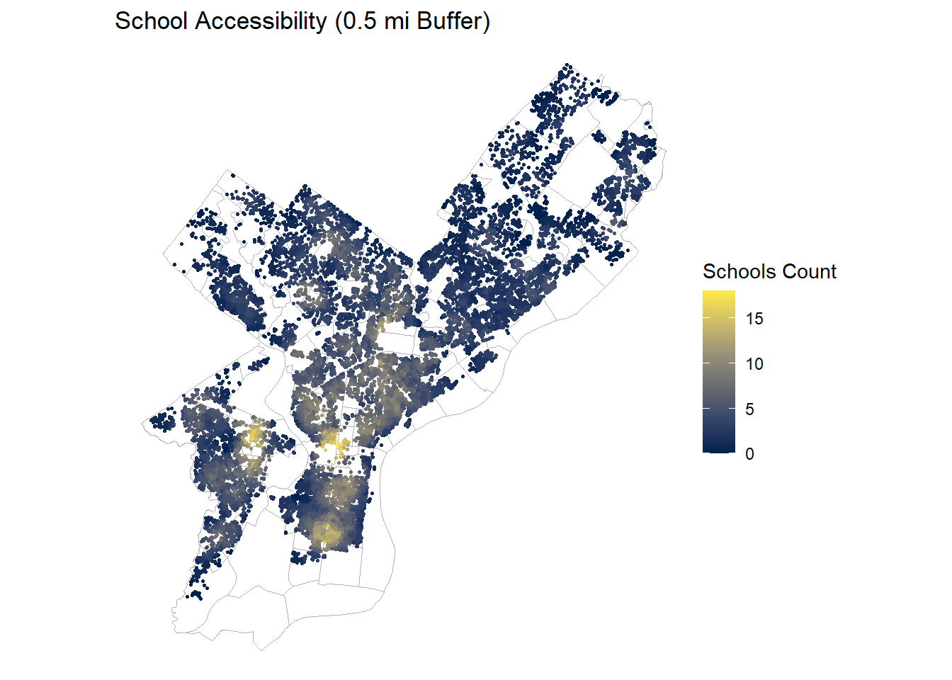
ggplot(OPA_points) +geom_sf(data = nhoods, fill =NA, color ="grey70", linewidth =0.3) +geom_sf(aes(color = schools_cnt_0p5mi), size =0.6) +scale_color_viridis_c(option ="cividis") +labs(title ="School Accessibility (0.5 mi Buffer)",color ="Schools Count") +theme_void()
Interpretation:
Transit proximity: Most parcels are within 500 ft of a stop, confirming strong transit coverage across Philadelphia.
Hospital proximity: Right-skewed distribution, consistent with limited facility count.
Parks access: Sparse exposure (mostly 0–1 within 0.25 mi), highlighting recreational inequities.
Crime exposure: Wide variation, clustered along high-density corridors; log-transformed to stabilize scale.
School proximity: Uniform urban coverage with typical parcels having 4-7 schools within 0.5 mi.
# function to check for statistically significant correlations between independent variablessig_corr <-function(dat, dep_var) {# remove the independent variable from the dataset dat_corr <- dat %>%select(-all_of(dep_var))# run a correlation matrix for the independent vars correlation_matrix <-rcorr(as.matrix(dat_corr)) values <- correlation_matrix$r vifs <-apply(values, 1, function(x){return(round(1/(1-abs(x)), 2)) }) values_df <- values %>%as.data.frame() vifs_df <- vifs %>%as.data.frame()# convert correlation coefficients and p-values to long format corCoeff_df <- correlation_matrix$r %>%as.data.frame() %>%mutate(var1 =rownames(.)) corVIF_df <- vifs %>%as.data.frame() %>%mutate(var1 =rownames(.)) corPval_df <- correlation_matrix$P %>%as.data.frame() %>%mutate(var1 =rownames(.))# merge long format data corMerge <-list( corCoeff_df %>%pivot_longer(-var1, names_to ="var2", values_to ="correlation") %>%as.data.frame(), corVIF_df %>%pivot_longer(-var1, names_to ="var2", values_to ="vif_factor") %>%as.data.frame(), corPval_df %>%pivot_longer(-var1, names_to ="var2", values_to ="p_value") %>%as.data.frame()) %>%reduce(left_join, by =c("var1", "var2"))# filter to isolate unique pairs, then rows with correlation > 0.5 and p < 0.05 corUnfiltered <- corMerge %>%filter(var1 != var2) %>%rowwise() %>%filter(var1 < var2) %>%ungroup() %>%as.data.frame() corFiltered <- corUnfiltered %>%filter(abs(vif_factor) >3& p_value <0.05) %>%arrange(desc(abs(correlation)))# save the raw correlation values and the filtered variable pairs final <-set_names(list(values_df, vifs_df, corUnfiltered, corFiltered),c("R2", "VIF", "AllCor", "SelCor"))return(final)}# create a dataset with just modeling variablesOPA_modelvars <- OPA_points %>%select(sale_price, total_livable_area, building_age, number_of_bedrooms, number_of_bathrooms, pop_totE, med_hh_incE, med_ageE, dist_nearest_transit_ft, dist_nearest_hospital_ft, parks_cnt_0p25mi, log1p_crime_cnt_0p5, schools_cnt_0p5mi, )# calculate VIFs and determine potentially troublesome correlations between variablesvif_check <-sig_corr(OPA_modelvars %>%st_drop_geometry(), dep_var ="sale_price")kable(vif_check[["VIF"]])
total_livable_area
building_age
number_of_bedrooms
number_of_bathrooms
pop_totE
med_hh_incE
med_ageE
dist_nearest_transit_ft
dist_nearest_hospital_ft
parks_cnt_0p25mi
log1p_crime_cnt_0p5
schools_cnt_0p5mi
total_livable_area
Inf
1.22
1.70
1.99
1.14
1.24
1.07
1.07
1.01
1.03
1.22
1.03
building_age
1.22
Inf
1.01
1.32
1.04
1.23
1.18
1.21
1.12
1.05
1.43
1.24
number_of_bedrooms
1.70
1.01
Inf
2.26
1.02
1.09
1.05
1.05
1.03
1.01
1.07
1.02
number_of_bathrooms
1.99
1.32
2.26
Inf
1.12
1.25
1.03
1.02
1.04
1.01
1.09
1.01
pop_totE
1.14
1.04
1.02
1.12
Inf
1.33
1.16
1.09
1.18
1.00
1.01
1.08
med_hh_incE
1.24
1.23
1.09
1.25
1.33
Inf
1.13
1.01
1.13
1.04
1.31
1.03
med_ageE
1.07
1.18
1.05
1.03
1.16
1.13
Inf
1.15
1.27
1.15
1.70
1.25
dist_nearest_transit_ft
1.07
1.21
1.05
1.02
1.09
1.01
1.15
Inf
1.25
1.11
1.72
1.44
dist_nearest_hospital_ft
1.01
1.12
1.03
1.04
1.18
1.13
1.27
1.25
Inf
1.10
1.85
1.66
parks_cnt_0p25mi
1.03
1.05
1.01
1.01
1.00
1.04
1.15
1.11
1.10
Inf
1.25
1.23
log1p_crime_cnt_0p5
1.22
1.43
1.07
1.09
1.01
1.31
1.70
1.72
1.85
1.25
Inf
2.46
schools_cnt_0p5mi
1.03
1.24
1.02
1.01
1.08
1.03
1.25
1.44
1.66
1.23
2.46
Inf
None of the variables tested have a significant VIF score that is above 3, indicating that there is little concern of multicollinearity in the models moving forward.
4 Model Building
4.1 Model 1: Structural Terms
Our first model uses structural property characteristics to build a multiple linear regression, regressing sale price on total livable area, number of bedrooms, number of bathrooms, and building age.
Call:
lm(formula = sale_price ~ total_livable_area + number_of_bedrooms +
    number_of_bathrooms + building_age, data = model1_data)

Residuals:
     Min       1Q   Median       3Q      Max
-1063434   -92640   -20598    58880  7759292

Coefficients:
                      Estimate Std. Error t value            Pr(>|t|)
(Intercept)         -11217.250  12625.853  -0.888               0.374
total_livable_area     221.516      5.126  43.217 <0.0000000000000002 ***
number_of_bedrooms  -34668.316   3239.669 -10.701 <0.0000000000000002 ***
number_of_bathrooms  70054.014   3967.307  17.658 <0.0000000000000002 ***
building_age           144.447    104.814   1.378               0.168
---
Signif. codes:  0 '***' 0.001 '**' 0.01 '*' 0.05 '.' 0.1 ' ' 1

Residual standard error: 233700 on 10324 degrees of freedom
Multiple R-squared:  0.2762,    Adjusted R-squared:  0.2759
F-statistic: 984.7 on 4 and 10324 DF,  p-value: < 0.00000000000000022
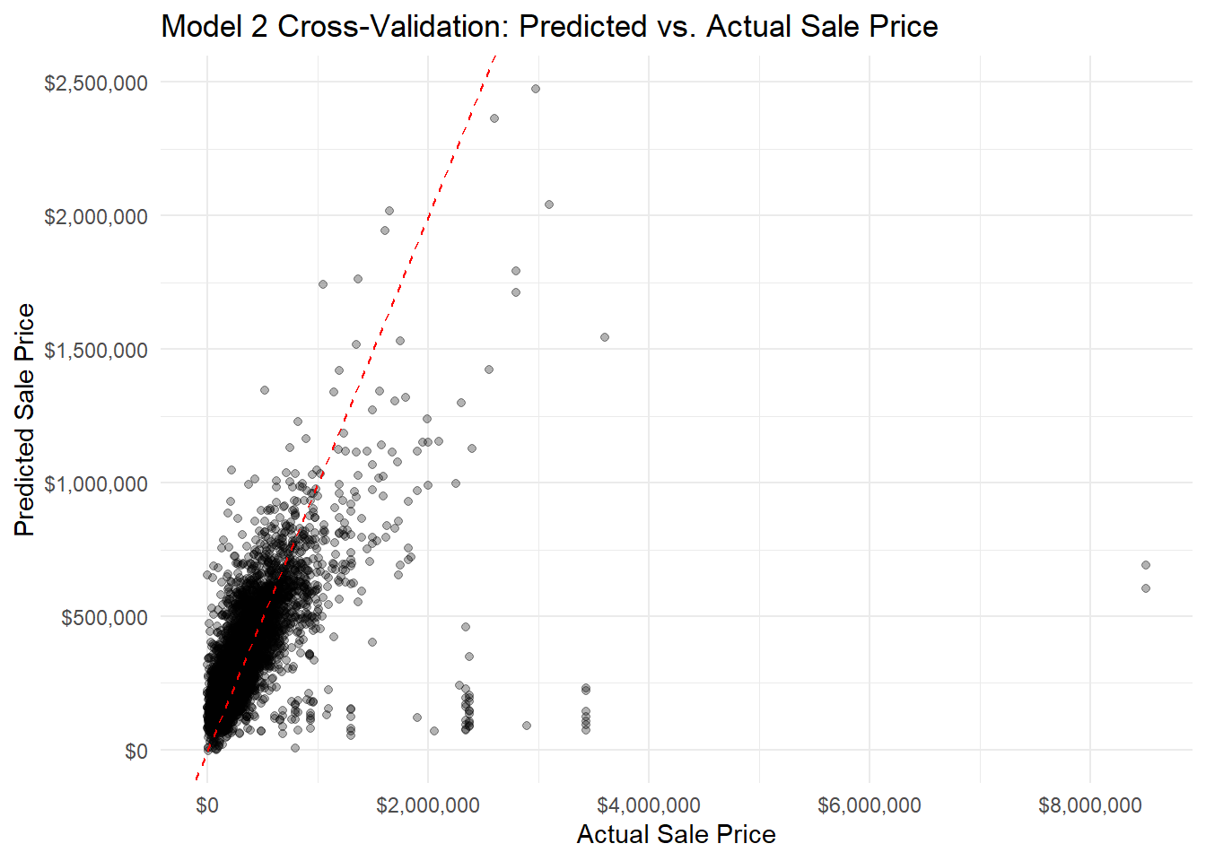
4.2 Model 2: Incorporation of Census Data
Our second model builds on the structural property characteristics regression by incorporating census tract–level variables, including population, median household income, and median age.
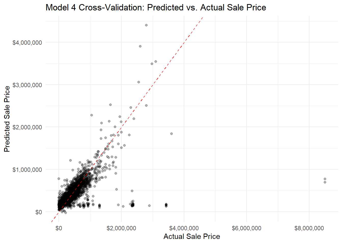
4.4 Model 4: Incorporation of Interactions and Fixed Effects
Code
# join data separately here to avoid conflicts with earlier code blocksOPA_points_copy <-left_join(OPA_points, neighbor_points %>%select(parcel_number, wealthy_neighborhood) %>%st_drop_geometry(),by ="parcel_number")
#there is only a premium on wealth neighborhood for total area, total livable area, and number of bathrooms that are significant. There is also a significant value for int_value_larea just from interacting the OPA data itsself which just assesses market value and size scalability.
4.5 Comparison of Model Performance
We can evaluate performance by conducting a 10-fold cross-validation of the 4 models, and comparing their RMSE, MAE, and \(R^2\).
# Model 1: Structural Features Onlymodel1_cv <-train( sale_price ~ total_livable_area + number_of_bedrooms + number_of_bathrooms + building_age,data =na.omit(OPA_points),method ="lm",trControl = train_control)model1_cv
Linear Regression

10329 samples
    5 predictor

No pre-processing
Resampling: Cross-Validated (10 fold)
Summary of sample sizes: 9295, 9297, 9296, 9297, 9296, 9296, ...
Resampling results:

  RMSE      Rsquared   MAE
  230140.4  0.2865262  115174.1

Tuning parameter 'intercept' was held constant at a value of TRUE
Linear Regression

10329 samples
    8 predictor

No pre-processing
Resampling: Cross-Validated (10 fold)
Summary of sample sizes: 9296, 9296, 9297, 9297, 9297, 9296, ...
Resampling results:

  RMSE      Rsquared   MAE
  215430.3  0.3799429  90217.97

Tuning parameter 'intercept' was held constant at a value of TRUE
Linear Regression

10329 samples
   13 predictor

No pre-processing
Resampling: Cross-Validated (10 fold)
Summary of sample sizes: 9295, 9297, 9295, 9295, 9296, 9298, ...
Resampling results:

  RMSE      Rsquared   MAE
  211021.2  0.4053308  90144.36

Tuning parameter 'intercept' was held constant at a value of TRUE
Linear Regression

10329 samples
   20 predictor

No pre-processing
Resampling: Cross-Validated (10 fold)
Summary of sample sizes: 9297, 9296, 9296, 9296, 9296, 9297, ...
Resampling results:

  RMSE      Rsquared   MAE
  194649.2  0.4958671  71748.91

Tuning parameter 'intercept' was held constant at a value of TRUE
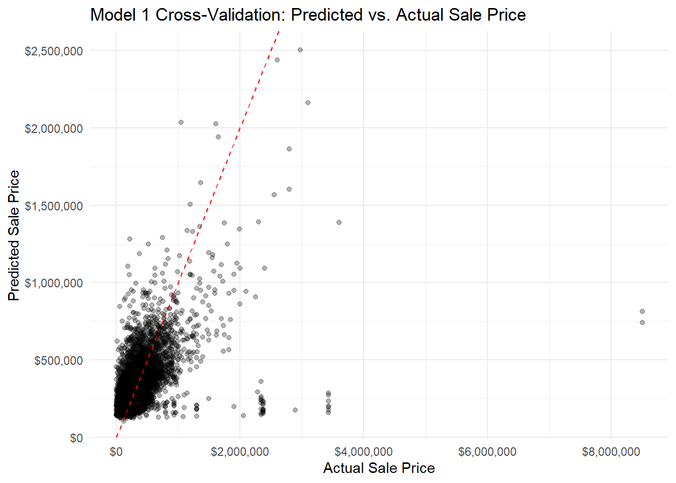
# plot predicted vs actual value plotsggplot(model1_cv$pred, aes(x = obs, y = pred)) +geom_point(alpha =0.3) +geom_abline(intercept =0, slope =1, color ="red", linetype ="dashed") +scale_x_continuous(labels =dollar_format()) +scale_y_continuous(labels =dollar_format()) +labs(title ="Model 1 Cross-Validation: Predicted vs. Actual Sale Price",x ="Actual Sale Price",y ="Predicted Sale Price" ) +theme_minimal()
Code
ggplot(model2_cv$pred, aes(x = obs, y = pred)) +geom_point(alpha =0.3) +geom_abline(intercept =0, slope =1, color ="red", linetype ="dashed") +scale_x_continuous(labels =dollar_format()) +scale_y_continuous(labels =dollar_format()) +labs(title ="Model 2 Cross-Validation: Predicted vs. Actual Sale Price",x ="Actual Sale Price",y ="Predicted Sale Price" ) +theme_minimal()
Code
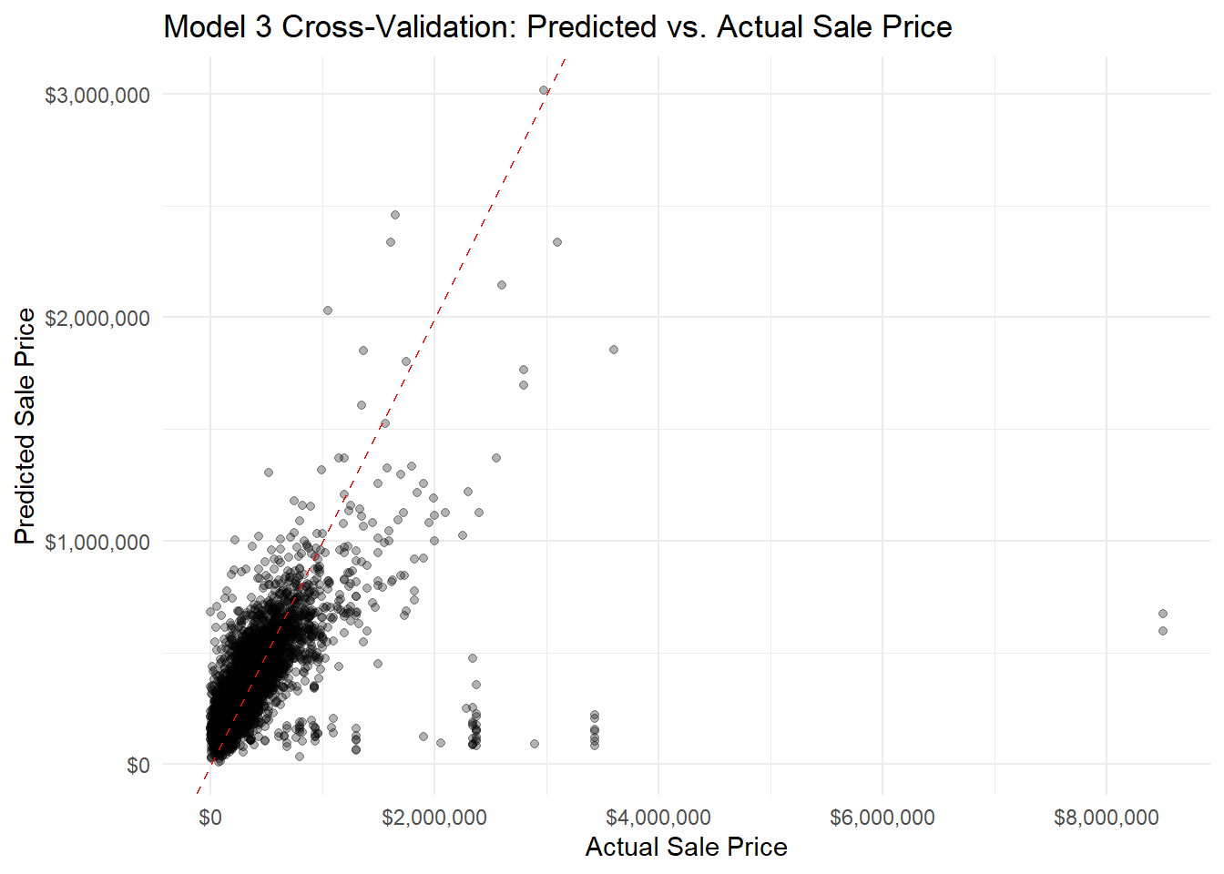
ggplot(model3_cv$pred, aes(x = obs, y = pred)) +geom_point(alpha =0.3) +geom_abline(intercept =0, slope =1, color ="red", linetype ="dashed") +scale_x_continuous(labels =dollar_format()) +scale_y_continuous(labels =dollar_format()) +labs(title ="Model 3 Cross-Validation: Predicted vs. Actual Sale Price",x ="Actual Sale Price",y ="Predicted Sale Price" ) +theme_minimal()
Code
ggplot(model4_cv$pred, aes(x = obs, y = pred)) +geom_point(alpha =0.3) +geom_abline(intercept =0, slope =1, color ="red", linetype ="dashed") +scale_x_continuous(labels =dollar_format()) +scale_y_continuous(labels =dollar_format()) +labs(title ="Model 4 Cross-Validation: Predicted vs. Actual Sale Price",x ="Actual Sale Price",y ="Predicted Sale Price" ) +theme_minimal()
5 Model Diagnostics
Code
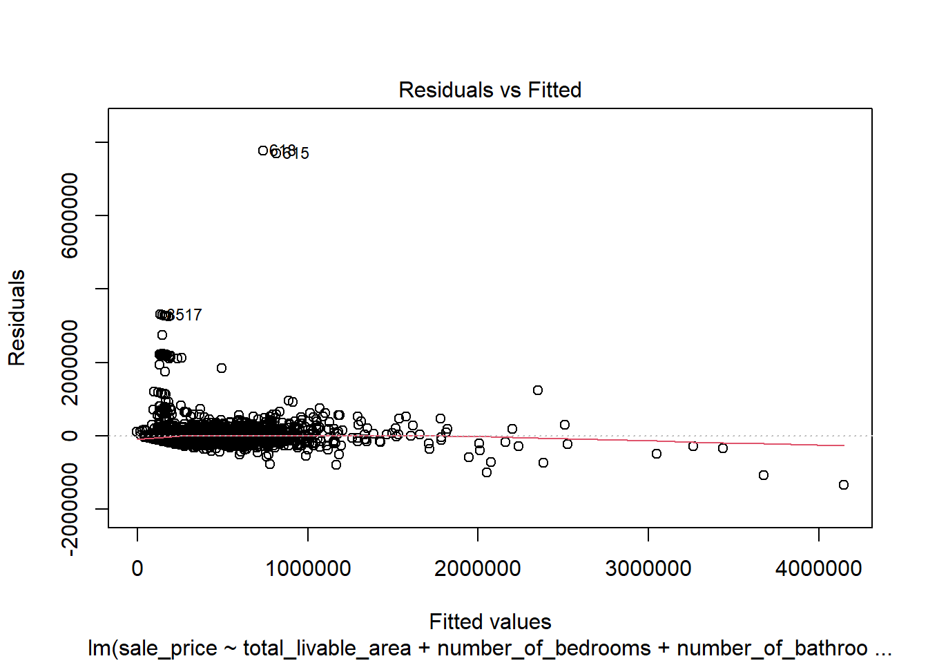
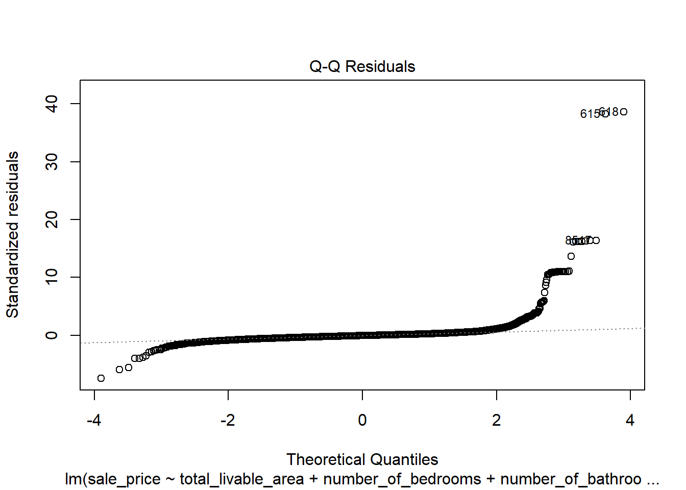
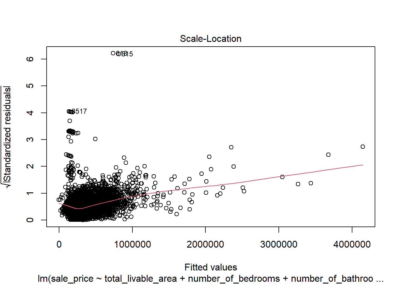
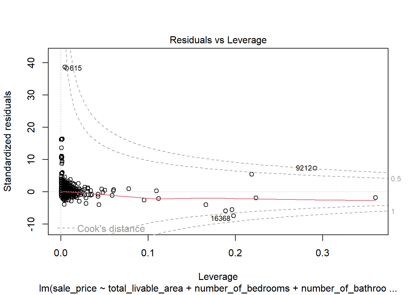
# create diagnostic plotsplot(model4)
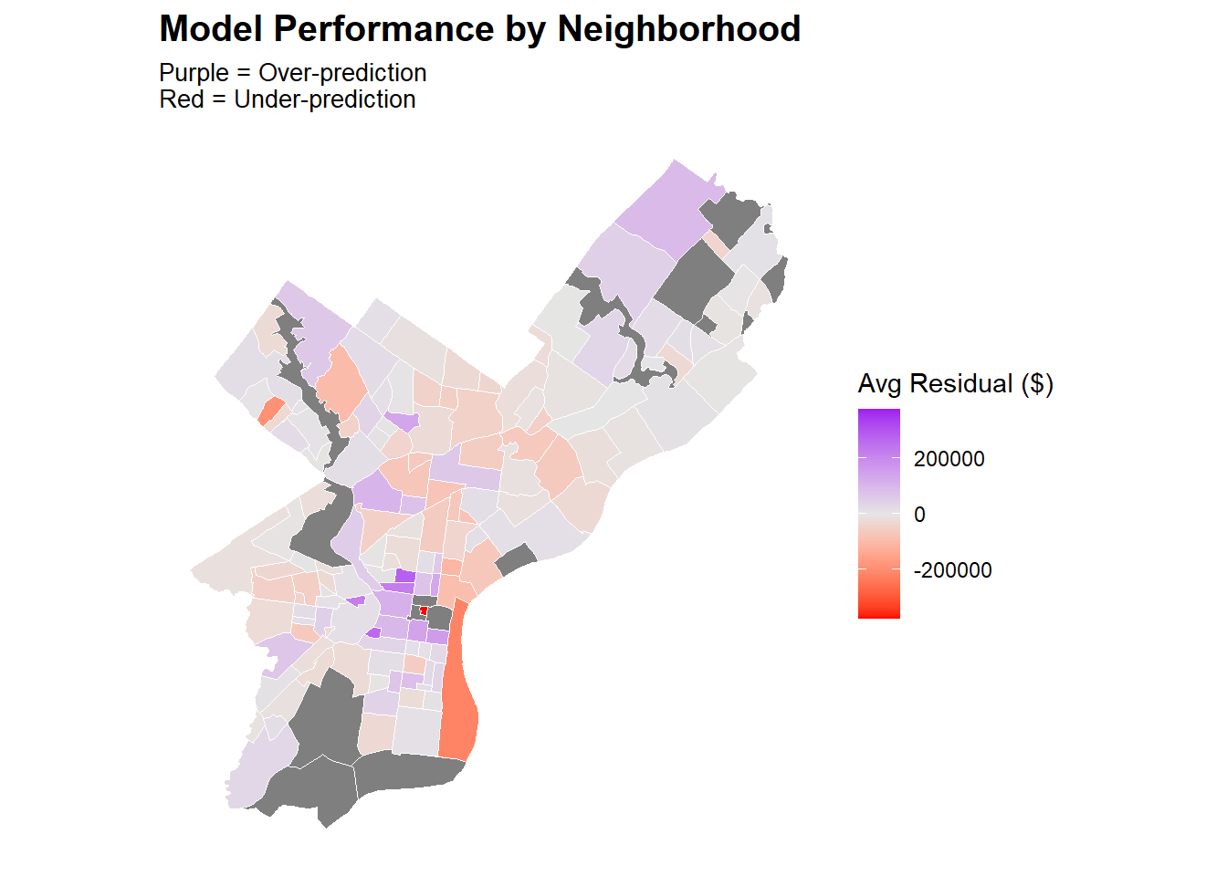
In the plot of residuals versus fitted values, the data largely displays a random distribution except for a spike in low sale price values. This indicates that the model might be poorly predicting for low sale price values as they don’t follow an entirely linear pattern. However, there was no visible cone shape in the data, which was a promising sign that this discrepancy was not due to a trend consistent across the entire dataset. This discrepancy is suspected to follow a neighborhood based spatial pattern, and that exploration is done below. The Q-Q plot indicates that residual values are not perfectly normally distributed, further confirming that the dataset does not seem to display a linear relationship around extreme values. However, an analysis of the residuals in a Cook’s Distance plot indicates that despite this lack of normality in the dependent variable, none of the observations are extraordinarily influential. These violations were therefore deemed mild enough to not warrant intervention.
The results of this map confirm suspicions of local parameters affecting sale price, and should guide future work as explained in the following section.
6 Conclusion and Recommendations
Our final model had an RMSE value of $195,093.2 and an MAE of $71,587.66. This was an improvement over previous models, where Model 1 had an RMSE value of $315,407.2 and an MAE of $146,134.04. Despite these improvements, these values are still extremely high relative to the current median household price in Philadelphia of approximately $232,000, according to Zillow. The strongest predicting features utilized in our model included whether the neighborhood a property had a median household income greater than $420,000 and could be considered wealthy (\(\beta\) = 47,309.230, p < 0.01), the number of bedrooms (\(\beta\) = 35,121.540, p < 0.01), and the number of bathrooms (\(\beta\) = 25,942.210, p < 0.01). Furthermore, our interaction term between wealthy neighborhood status and the number of bathrooms proved to also strongly influence the model output (\(\beta\) = 22,639.990, p < 0.01), indicating that properties in wealthier neighborhoods that have additional bathrooms tend to gain a stronger sale price premium compared to properties in non-wealthy neighborhoods.
Sale prices in Philadelphia do not seem to entirely follow a linear relationship, particularly among lower-priced homes. This resulted in limited prediction potential for properties with lower sale prices. This could produce potential equity issues related to pricing homes of lesser value and those in lower-income neighborhoods that are impacted by surrounding properties. Many of the variables used were simply aggregated without being weighted, such as how the count of crime incidents within a half-mile does not take into account the severity of such events or how the quality of parks within a quarter-mile of a property is not considered. This could over- or under-emphasize these variables in the model.